Examples

I illustrate the residual migration technique with one synthetic and one real data example.

The first example is a simple 2D model with a 4 dipping reflectors embedded in a velocity model which varies smoothly both as a function of horizontal position and as a function of depth. synt.model shows, from top to bottom, the slowness model, the reflectivity model and the zero offset of the 2D modeled data. The data were generated with a wavefield-continuation operator (24; 82; 86). The maximum offset of the simulated data is 2.56 km, and the velocity ranges between 2.0 km/s in the upper left corner to 2.4 km/s in the lower right corner.

 

synt.model Figure 1 Synthetic model. From top to bottom, slowness model, reflectivity model and the zero offset section of the modeled 2D prestack data.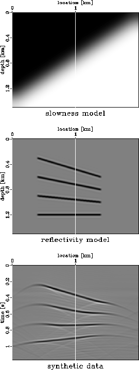

To test the prestack Stolt residual migration, I migrate the synthetic data using wavefield-continuation with the mixed-domain split-step Fourier method. The tests are carried out using two velocity models: the correct velocity, and an incorrect velocity model which is obtained from the correct one by scaling with a factor of 0.8.

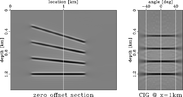
synt.RC.zhm shows the image obtained using the correct velocity model. The left panel represents the zero offset section of the image obtained by 2D prestack downward-continuation migration. The right panel represents a common image gather in the angle domain (adcig), extracted at the horizontal location x=1 km.

 

synt.RC.zhm
Figure 2 Migrated image (zero offset section) and angle-domain CIG for the synthetic data in synt.model obtained using the correct velocity model.

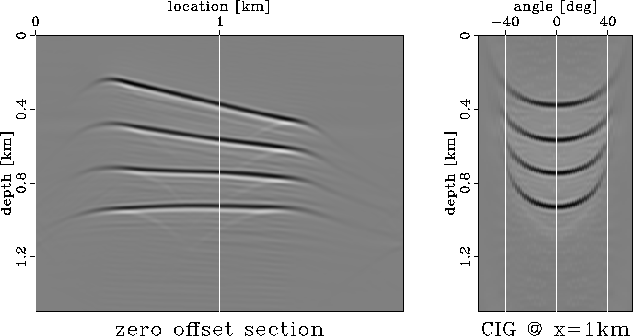
synt.R0.zhm shows the image obtained using the incorrect velocity model. Since this velocity is smaller than the correct one, the image is strongly undermigrated, and the events in the angle-domain common image gathers bend strongly upward.

 

synt.R0.zhm
Figure 3 Migrated image (zero offset section) and angle-domain CIG for the synthetic data in synt.model obtained using the incorrect velocity model scaled by $\rho=0.8$.

synt.R0.srm shows the result of applying Stolt residual migration using the correct velocity ratio ($\rho=0.8$) to the undermigrated image in synt.R0.zhm. The result is a well focused image, with reasonably flat angle gathers. This result shows that, although only approximate for variable velocity media, the method outlined in this section can successfully operate on depth migrated images despite the assumption of constant velocity made in the derivation. Of course, there is no guarantee that the method will be successful on arbitrary velocity models. However, on fairly smooth models, Stolt residual migration can at least indicate the direction of the changes that improve the migrated image.

 

synt.R0.srm
Figure 4 Residually migrated image (zero offset section) and angle-domain CIG for the synthetic data in synt.model obtained from the image in synt.R0.zhm after residual migration with the correct velocity ratio $\rho=0.8$.

The second example concerns a real dataset from a complex salt dome region in the North Sea (111). This dataset was donated to SEP by Elf and it is part of the SEP data library. saltreal.raw shows a zero-offset section obtained by 2D prestack downward-continuation migration. We can clearly distinguish the salt body and the sediment layers. However, the area under the salt overhang is not imaged correctly, mostly due the inaccuracies in the velocity model (111).

 

saltreal.raw
Figure 5 Migrated image of the North Sea data. The area of interest is surrounded by the thick box.

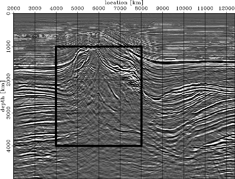The errors in this image are too complex for a simple algorithm like the one outlined in this section to be fully successful. We cannot hope to recover the exact structure under the salt overhang just by residual migration. However, we can use the speed of such an algorithm to investigate whether any other piece of the image can be brought in focus, and to determine roughly in which direction we need to modify the velocity model.

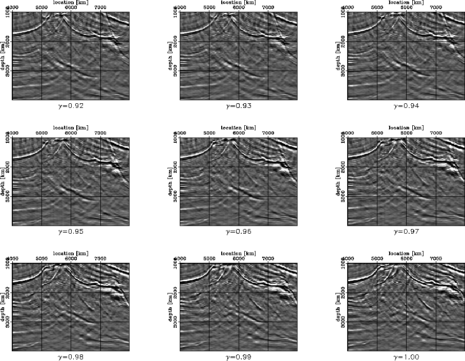
saltreal.srm shows the result of residual migration. Each one of the 9 panels corresponds to the box depicted in saltreal.raw. The images are obtained for various values of the parameter $\rho$ ranging from $\rho=1.0$ to $\rho=0.92$ as labeled in the figure.

We can observe several things: the top of salt, which was not well focused in the original image ($\rho=1.0$), is better focused in some of the panels corresponding to lower values of the parameter $\rho$;the salt overhang is brought into much better focus, particularly in the panel corresponding to $\rho=0.94$ around x=6000 and z=3000; the sediments that are practically impossible to track in the original image are more coherent and can be traced much deeper under the salt overhang on the image corresponding to $\rho=0.94$.

 

saltreal.srm
Figure 6 Prestack Stolt residual migration for a range of velocity ratio parameters ($\rho$) from 1.0 to 0.92. All panels correspond to the box in saltreal.raw.

saltreal.constant is a comparison between the original image ($\rho=1.00$, top panel) and the image obtained by prestack Stolt residual migration that best resolves the salt overhang and sediments underneath ($\rho=0.94$, bottom panel). For comparison, the middle panel shows an image obtained by residual moveout which also shows an improvement over the original image, but not as good as the one obtained by residual migration. This is understandable, since residual moveout does not allow energy to move between midpoints, while residual migration does.

 

saltreal.constant Figure 7 A comparison of the original image (top panel) with the improved images obtained by residual moveout (middle panel) and the image after residual migration with a constant velocity ratio parameter 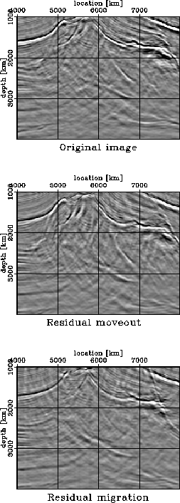$\rho=0.94$(bottom panel). All panels correspond to the box in saltreal.raw.

Finally, if we carefully analyze the images in saltreal.srm, we can observe that various parts of the image are in good focus at different values of the ratio parameter $\rho$. This leads to the conclusion that none of the panels in saltreal.srm alone can serve as an improved image at all locations in the image. One possible solution to this problem is to create a smooth interpolation map which slices through the various images at different values of $\rho$ for every location in the image. saltreal.variable shows such a result: the top and middle images are respectively the original and improved images for variable $\rho$, and the bottom panel is the interpolation map used to extract the middle panel.

 

saltreal.variable Figure 8 A comparison of the original image (top panel) with the image obtained by residual migration (middle panel) with a spatially varying 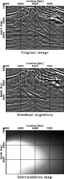$\rho$.The velocity ratio parameter $\rho$ is ranging from 0.91 to 1.00 (bottom panel). All panels correspond to the box in saltreal.raw.