Test results

I tested this method on the Madagascar satellite data set with increasingly sparse missing data. I found that this method estimated a 2D PEF that is comparable to a 2D PEF estimated on dense data when the sparse data was 67 percent unknown. For input data that was more sparse than that, the method failed.

 

dense_sparse
Figure 1 Left is the dense data in the overlapping region. Right is the sparse data.

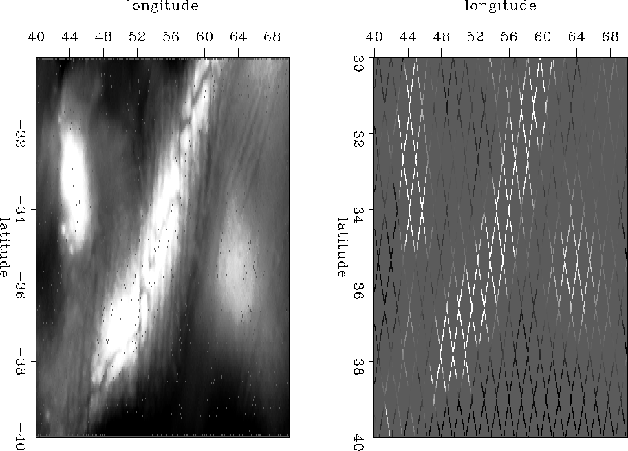
The data consists of two overlapping datasets. One is densely sampled and one is sparsely sampled. I chose to work in the overlapping region. On the left side of Figure is the dense data in the southern half of the Madagascar data. The right of the figure is the sparse data overlapping the dense data.

 

dense_fill
Figure 2 Left is the dense data with it few empty bins filled with a laplacian. Right is the same data roughened with the helical derivative.

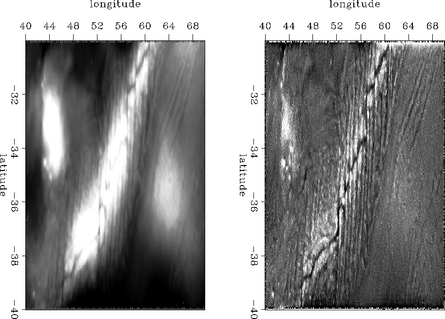Figure is the dense data after its few empty bins have been filled with a laplacian. The right side has been roughened with the helical derivative.

 

comp_imp
Figure 3 Left is the impulse response of the inverse full 2D PEF estimated on southern dense region after the few remaining bins have been filled using a 2D gradient as regularization. Right is the impulse response of the inverse helical derivative. This is the starting solution for the sparse 2D PEF estimation.

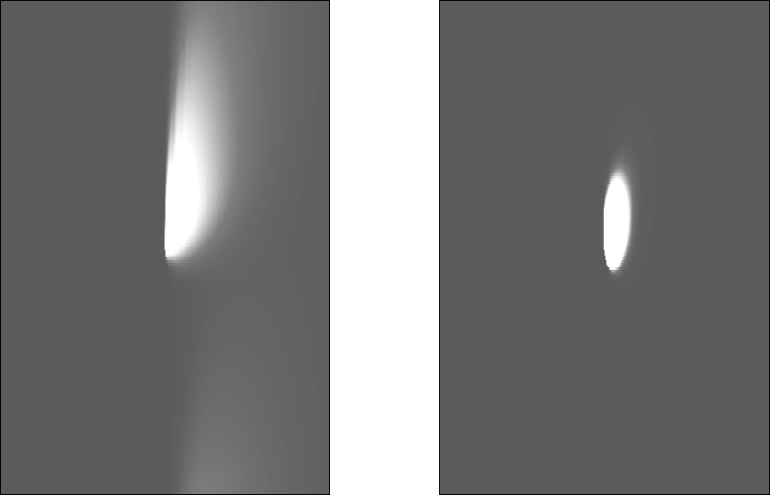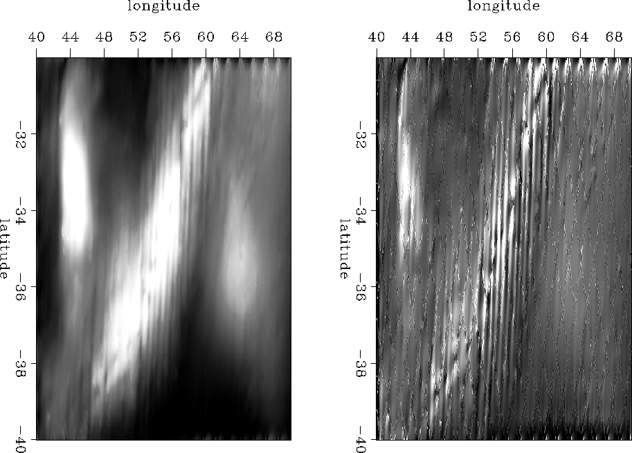
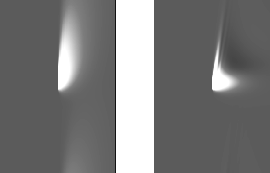
I began with the densely sampled data and gradually threw away data. As I threw out data, I compared the impulse response of the inverse 10 by 10 PEF estimated on the dense data to the impulse response of the inverse PEF estimated using the approach described in the paper. The left side of Figure is the impulse response wrapped on the helix of the inverse PEF estimated on the dense data in Figure . Notice that it has a similar character to data it is trying to emulate. This is the result that the sparse 2D PEF is hoping to achieve.

For nonlinear problems, the initial solution is extremely important. Thus far, I have used only the helical derivative Claerbout (1999). In the future, other starting solutions may improve the results, such as the solution used in Curry (2004b). In the right side of Figure , is the impulse response of the inverse helical derivative.

 

data_mask.4.wide Figure 4 This is the map to be interpolated. The tracks have been made thicker therefore it is less sparse than the original sparse tracks.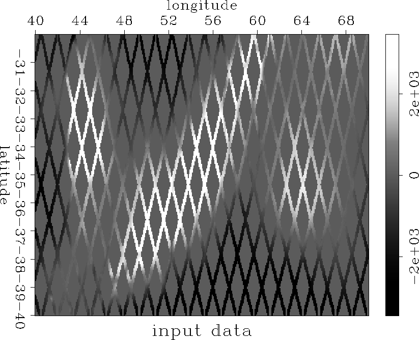

Figure shows thicker tracks than the original sparse data shown on the right side of Figure . This has 2.6 times as many non-zero values as the original sparse data.

 

coef_fold.4.wide Figure 5 A coefficient fold map for the tracks in Figure with a 10 by 10 filter. The value indicates the number of coefficients of the filter that are on known data at each location in the model.

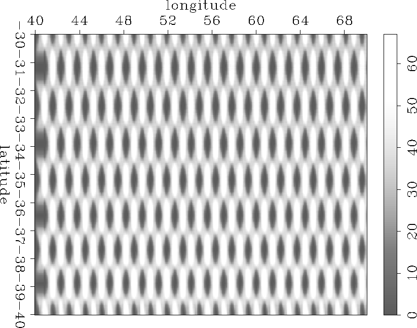Figure shows the coefficient fold map for a 10 by 10 filter on the sparse data in Figure . The number of coefficients that are on known data at each point in the model can be thought of as the coefficient fold. A coefficient fold map can easily be created by packing the filter with all ones and setting the known data in the model to ones and the unknown to data to zeros. The output of the convolution is a coefficient fold map.

 

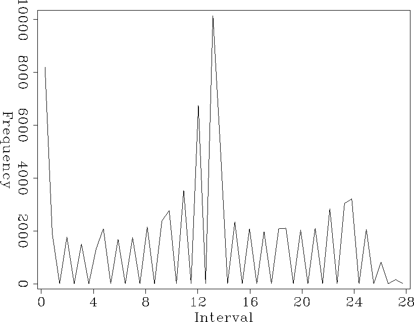
histo.4 Figure 6 A histogram of the values in the coefficient fold map in Figure . Notice that most of the filter locations have about 33 out of about 98 coefficients on known data. The areas with the highest (50-65) are located where the tracks cross.

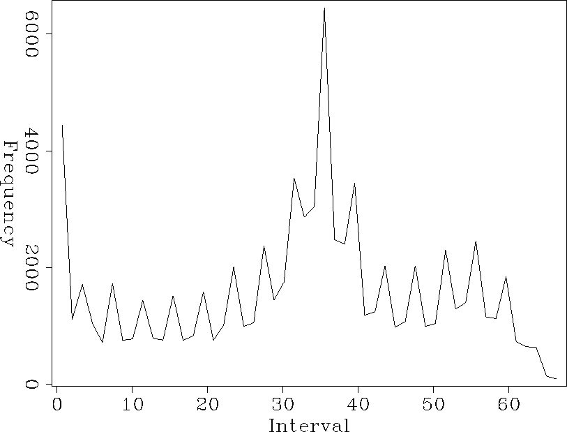In Figure is a histogram of the convolution map in Figure . For this 10 by 10 PEF, there are 98 coefficients. It can be seen in the histogram that the maximum coefficient fold is approximately 67. This means that at those locations 31 filter coefficients are on unknown data. Also, most of the filter locations have about 33 coefficients on known data, 65 coefficients on unknown data. In this case, I set the first minimum fold parameter to 60, solved for the filter and missing data. Then set the minimum fold parameter to 50 and repeated until all of the data was used.

 

comp_imp2.4
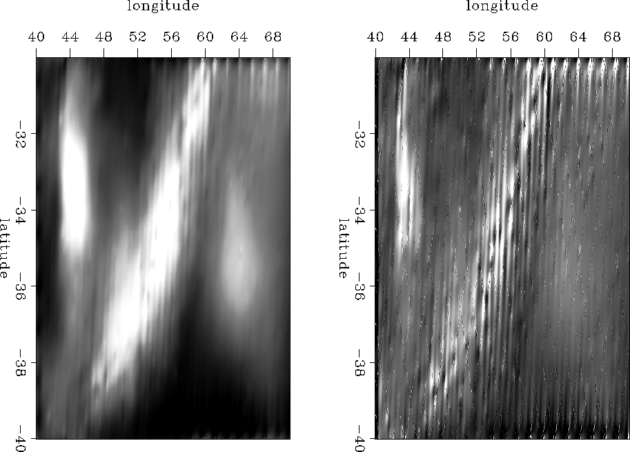
Figure 7 Left is the impulse response of the inverse 2D PEF estimated on the dense data in left of Figure . Right is the impulse response of the inverse 2D PEF estimated on the sparse tracks in Figure .

Figure compares the impulse responses of the inverse PEF of the full 2D PEF on the left to the 2D PEF estimated on the sparse tracks from Figure on the right. Although they are not exactly the same, they are similar. The sail shape possibly results from the PEF's ability to capture the narrow ridges trending almost north and the entire submerged mountain range trending west and its inability to capture the central spreading ridge trending northeast.

 

hel.2d.4.fill
Figure 8 Left is the result of filling the sparse tracks in Figure with a full 2D PEF estimated on the dense data in left side of Figure . Right is roughened with the helical derivative.

 

recursive_pef.4.fill
Figure 9 Left is the result of estimating a sparse 2D PEF on the sparse tracks in Figure and filling in the same data. Right is roughened with the helical derivative. Notice the similarity to Figure .

Another comparison to evaluate the quality of the result is to inspect the filled data. Figure is the sparse tracks in Figure filled with the full 2D PEF estimated on the dense data. Figure is the sparse tracks in Figure filled with the 2D PEF estimated on the sparse tracks themselves. In general, this method adequately fills the missing data, only showing some weakness in capturing the main spreading ridge feature.

 

coef_fold Figure 10 A coefficient fold map for the sparse tracks with a 10 by 10 filter. The value indicates the number of coefficients of the filter that are on known data at each location in the model.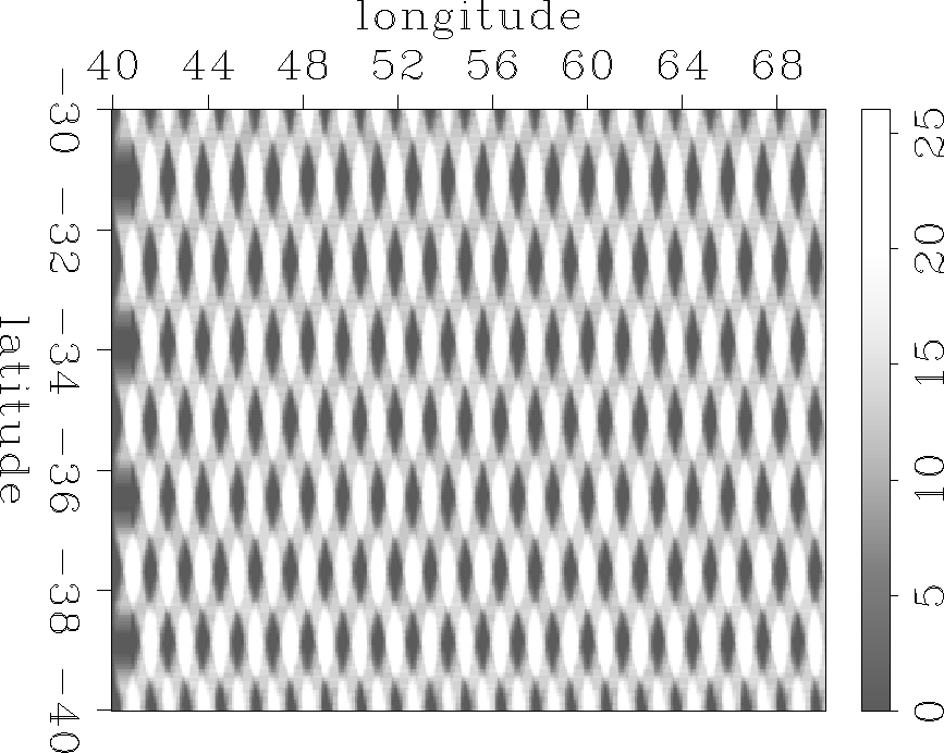

 

histo.1 Figure 11 A histogram of the values in the coefficient fold map in Figure . Notice that most of the filter locations have about 13 out of about 98 coefficients on known data.

 

comp_imp2.1
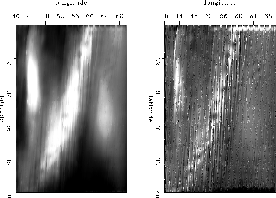
Figure 12 Left is the impulse response of the inverse 2D PEF estimated on the dense data in left of Figure . Right is the impulse response of the inverse 2D PEF estimated on the sparse tracks in the right of Figure . The two impulse responses are noticeably different.

If the data is too sparse, this method fails. Estimating a PEF on the original sparse tracks on the right side of Figure illustrates this. First, we recalculate a new coefficient fold map shown in Figure . Analysis of the histogram in Figure reveals that this data is indeed very sparse. Then, Figure compares the impulse responses. The sparse 2D PEF on the right does a very poor job of matching the desired response on the left. Comparison of the filled results in Figures and further demonstrate the sparse 2D PEF inability to capture much of the high frequencies.

 

hel.2d.1.fill
Figure 13 Left is the result of filling the sparse tracks in the right of Figure with a full 2D PEF estimated on the dense data in left side of Figure . Right is roughened with the helical derivative.

 

recursive_pef.1.fill
Figure 14 Left is the result of estimating a sparse 2D PEF on the sparse tracks in the right Figure . Right is roughened with the helical derivative. Unfortunately, it is not able to capture the higher frequency nature of the data as captured by the full 2D PEF result shown in Figure .