Explicit correction operator

Explicit extrapolation operators have been proved useful in isotropic wavefield extrapolation Hale (1991); Hale (1991); Blacquiere et al. (1989); Holberg (1988); Thorbecke (1997). They are also applied in wavefield extrapolation for TI media Zhang et al. (2001). For an isotropic or VTI medium, the extrapolation operator is symmetric and can be approximated by a cosine function series. For a tilted TI medium, k_z is not an even function of k_x, and the extrapolation operator is asymmetric. Thus, we need both the sine and cosine function series to approximate the correction operator in the wavenumber domain. 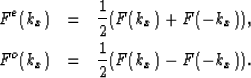In equation (6), F(k_x) is not an even function, but can be divided F(k_x) into two parts: even function F^e(k_x) and odd function F^o(k_x),

$$\begin{eqnarray} F^e(k_x)&=&\frac{1}{2}(F(k_x)+F(-k_x)),\\ F^o(k_x)&=&\frac{1}{2}(F(k_x)-F(-k_x)).\end{eqnarray}$$ (8) (9)

To design the explicit correction operator, we specify F^e(k_x) in the form  

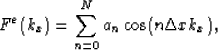$$F^e(k_x)=\sum_{n=0}^{N}a_n\cos(n\Delta x k_x),$$ (10)

and F^o(k_x) in the form  

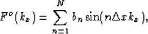$$F^o(k_x)=\sum_{n=1}^{N}b_n\sin(n\Delta x k_x),$$ (11)

where a_n,b_n are complex coefficients. These coefficients can be determined by the following weighted least-squares fitting goals:  

$${\bf W}({\bf Aa}-{\bf f^e}) \approx {\bf 0},$$ (12)

 

$${\bf W}({\bf Bb}-{\bf f^o}) \approx {\bf 0},$$ (13)

where

$${\bf a}=(a_0,a_1,\cdots, a_N)^T,$$

$${\bf b}=(b_1,b_2, \cdots, b_N)^T.$$

${\bf A}$ is an $(M+1)\times (N+1)$ matrix with elements ${A}_{mn}=\cos(mn\Delta k_x\Delta x)$, $m=0,1,2, \cdots, M$, and $n=0,1,2, \cdots, N$. ${\bf B}$ is an $M\times N$ matrix with elements ${B}_{mn}=\sin(mn\Delta k_x\Delta x)$, $m=1,2, \cdots, M$, and $n=1,2, \cdots, N$. ${\bf f^e}$ is a vector with elements $F^e(m\Delta k_x)$, $m=0,1,2, \cdots, M$. ${\bf f^o}$ is a vector with elements $F^o(m\Delta k_x)$, $m=1,2, \cdots, M$. ${\bf W}$ is a diagonal matrix with proper weights for the wavenumber k_x. One way to solve the fitting goal (12) is to do QR decomposition Golub and Van Loan (1996) of the matrix ${\bf WA}$:${\bf WA}={\bf QR}$, where ${\bf Q}$ is an orthogonal matrix and ${\bf R}$ is an upper triangular matrix. Then the coefficient vector ${\bf a}$ is given by

$${\bf a}={\bf R}^{-1}{\bf Q}^T{\bf Wf^e}.$$ (14)

We can solve the fitting goal in equation (13) and obtain the coefficient vector ${\bf b}$ in the same way. After we have the coefficient vectors ${\bf a}$ and ${\bf b}$, we can combine them into the coefficients for the explicit correction operator. From Fourier transform theory, it is well known that the inverse Fourier transform of the function $\cos(n\Delta x k_x)$ and $\sin(n\Delta x k_x)$ are:

$$\begin{eqnarray} {\mathcal{F}}^{-1}\{\cos(n\Delta x k_x)\}&=&\frac{1}{2}(\delta(... ... k_x) \}&=& \frac{1}{2i}(\delta(x-n\Delta x)-\delta(x+n\Delta x)).\end{eqnarray}$$ (15) (16)

Thus, the inverse Fourier transform of the function $a_n \cos(n\Delta x k_x)+b_n \sin(n\Delta x k_x)$ is

$${\mathcal{F}}^{-1}\{ a_n \cos(n\Delta x k_x)+b_n \sin(n\Delt... ...n)\delta(x-n\Delta x)+\frac{1}{2}(a_n-ib_n)\delta(x+n\Delta x).$$

Therefore, the explicit correction operator is:

$$(c_{-N},c_{-(N-1)},\cdots, c_{-1},c0,c_1,\cdots, c_{(N-1)}, c_{N}),$$ (17)

where c₀=a₀, and

$$c_{-n}=\frac{1}{2}(a_n-ib_n), \ \ n=1,2,\cdots, N,$$

$$c_n=\frac{1}{2}(a_n+ib_n), \ \ n=1,2,\cdots, N.$$

In 3-D, based on the following trigonometric identity,

$$\cos (n \theta)=2\cos(\theta)\cos[(n-1)\theta]-\cos[(n-2)\theta],$$ (18)

we can run McClellan transformations Hale (1991); McClellan and Chan (1977); McClellan and Parks (1972) for the cosine terms. Similarly, based on the trigonometric identity:

$$\sin (n \theta)=2\cos(\theta)\sin[(n-1)\theta]-\sin[(n-2)\theta],$$ (19)

we can design a recursive operator similar to McClellan transformations for the sine terms.

 

ico
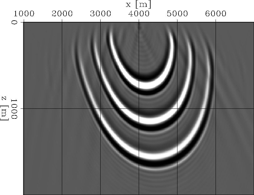
Figure 1 Impulse response of isotropic phase-shift with an anisotropic correction operator.

 

icoffd
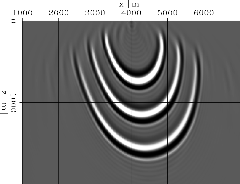
Figure 2 Impulse response of isotropic FFD with an anisotropic correction operator.

 

phsift
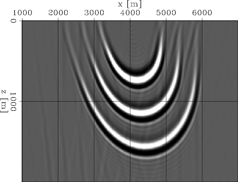
Figure 3 Impulse response of anisotropic phase-shift.