![[*]](http://sepwww.stanford.edu/latex2html/cross_ref_motif.gif) ). We choose a target zone (indicated with the "target" box in Figure
). We choose a target zone (indicated with the "target" box in Figure ![[*]](http://sepwww.stanford.edu/latex2html/cross_ref_motif.gif) ) to see the effects of the faults on the Hessian.
) to see the effects of the faults on the Hessian.
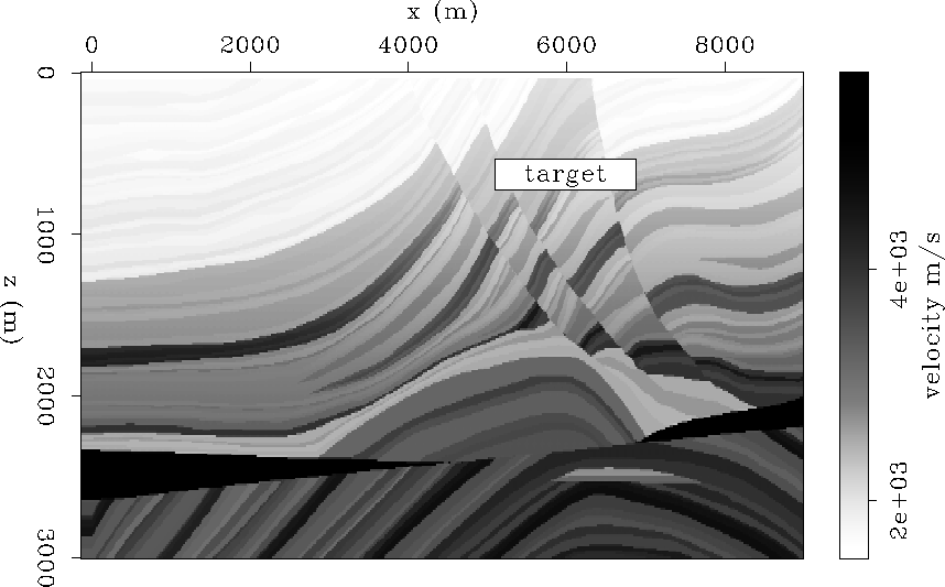
The Marmousi synthetic data set Bourgeois et al. (1991) was first released as a blind test for velocity estimation. It has become a popular testbed for migration algorithms. Its structural style is dominated by growth faults, which arise from salt creep and give rise to the complicated velocity structure in the upper part of the model (Figure ![[*]](http://sepwww.stanford.edu/latex2html/cross_ref_motif.gif) ). We choose a target zone (indicated with the "target" box in Figure
). We choose a target zone (indicated with the "target" box in Figure ![[*]](http://sepwww.stanford.edu/latex2html/cross_ref_motif.gif) ) to see the effects of the faults on the Hessian.
) to see the effects of the faults on the Hessian.
 |
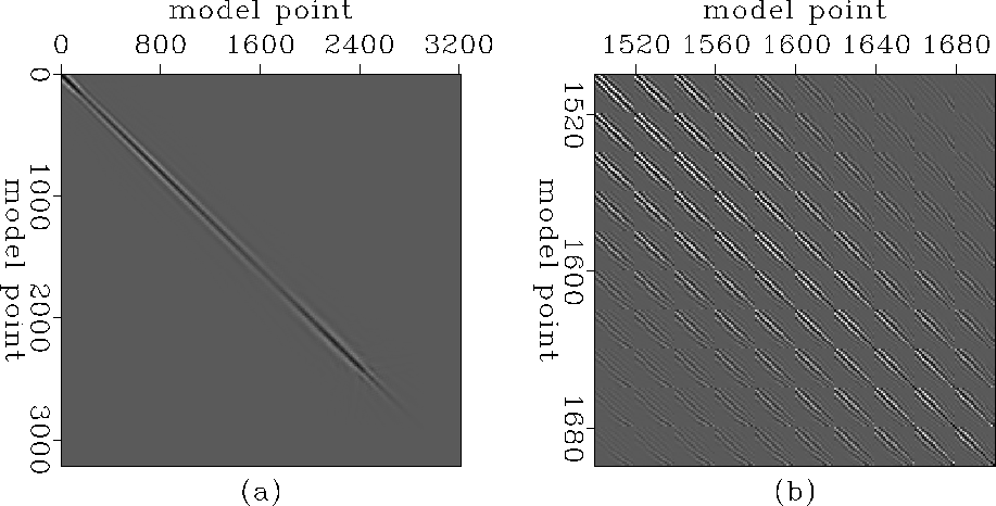
Figures ![[*]](http://sepwww.stanford.edu/latex2html/cross_ref_motif.gif) a and
a and ![[*]](http://sepwww.stanford.edu/latex2html/cross_ref_motif.gif) b show the Hessian matrix of the Marmousi model. Notice the banded nature of the matrix (Figure
b show the Hessian matrix of the Marmousi model. Notice the banded nature of the matrix (Figure ![[*]](http://sepwww.stanford.edu/latex2html/cross_ref_motif.gif) b), with most of the energy in the main diagonal (Figure
b), with most of the energy in the main diagonal (Figure ![[*]](http://sepwww.stanford.edu/latex2html/cross_ref_motif.gif) a). There are changes of the energy in the diagonal, but not as strong as for the Sigsbee model case.
a). There are changes of the energy in the diagonal, but not as strong as for the Sigsbee model case.
 |
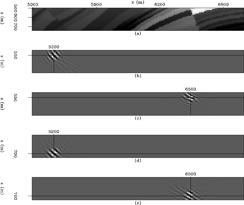
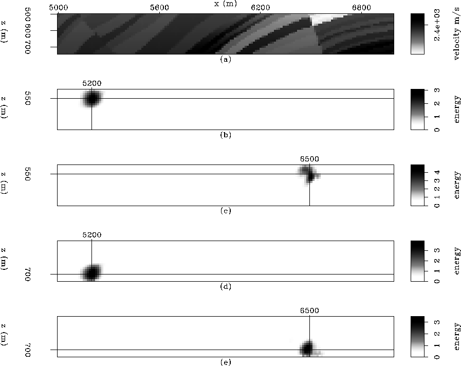
We fixed four points to see the lines of the Hessian corresponding to different geological features in the model. Figures ![[*]](http://sepwww.stanford.edu/latex2html/cross_ref_motif.gif) and
and ![[*]](http://sepwww.stanford.edu/latex2html/cross_ref_motif.gif) show the Hessian and the envelope of the Hessian, respectively. The envelope of the Hessian (Figure
show the Hessian and the envelope of the Hessian, respectively. The envelope of the Hessian (Figure ![[*]](http://sepwww.stanford.edu/latex2html/cross_ref_motif.gif) ) shows clearly the main features of interest.
) shows clearly the main features of interest.
 |
Figure ![[*]](http://sepwww.stanford.edu/latex2html/cross_ref_motif.gif) a shows a close-up of the velocity model in the area where the target-oriented Hessian was computed. Figure
a shows a close-up of the velocity model in the area where the target-oriented Hessian was computed. Figure ![[*]](http://sepwww.stanford.edu/latex2html/cross_ref_motif.gif) b shows point 1, with coordinates
b shows point 1, with coordinates ![]() . Since this point in the model is well illuminated, the resulting ellipse looks similar to the constant-velocity ellipses. Figure
. Since this point in the model is well illuminated, the resulting ellipse looks similar to the constant-velocity ellipses. Figure ![[*]](http://sepwww.stanford.edu/latex2html/cross_ref_motif.gif) c shows point 2, with coordinates
c shows point 2, with coordinates ![]() . Notice that this point is close to a fault, producing a distortion to the ellipse shape. Figure
. Notice that this point is close to a fault, producing a distortion to the ellipse shape. Figure ![[*]](http://sepwww.stanford.edu/latex2html/cross_ref_motif.gif) d shows point 3, with coordinates
d shows point 3, with coordinates ![]() ; as with point 1, the ellipse is not distorted. Finally, Figure
; as with point 1, the ellipse is not distorted. Finally, Figure ![[*]](http://sepwww.stanford.edu/latex2html/cross_ref_motif.gif) e shows point 4, with coordinates
e shows point 4, with coordinates ![]() . This point is also close to the fault, but the velocity contrast across the fault is smaller, producing less distortion than in the point 3 case.
. This point is also close to the fault, but the velocity contrast across the fault is smaller, producing less distortion than in the point 3 case.
 |