


It is possible to explicitly compute the Hessian for small models, or if a target-oriented strategy is followed. We created a synthetic data set assuming a land-type acquisition geometry: the shots were positioned every ![]() from
from ![]() to
to ![]() , keeping fixed receivers from
, keeping fixed receivers from ![]() to
to ![]() . Figures
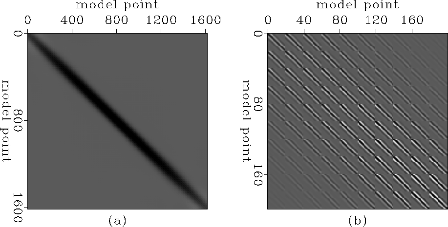
. Figures ![[*]](http://sepwww.stanford.edu/latex2html/cross_ref_motif.gif) a and b show the Hessian matrix of the constant-velocity model. Notice the banded nature of the matrix (Figure b), with most of the energy in the main diagonal Chavent and Plessix (1999). At the extremes of the diagonal the amplitudes become dimmer (Figure a) indicating points of lower illumination at the extremes of the acquisition.
a and b show the Hessian matrix of the constant-velocity model. Notice the banded nature of the matrix (Figure b), with most of the energy in the main diagonal Chavent and Plessix (1999). At the extremes of the diagonal the amplitudes become dimmer (Figure a) indicating points of lower illumination at the extremes of the acquisition.
 |
a.


For a fixed point ![]() , each line of the Hessian
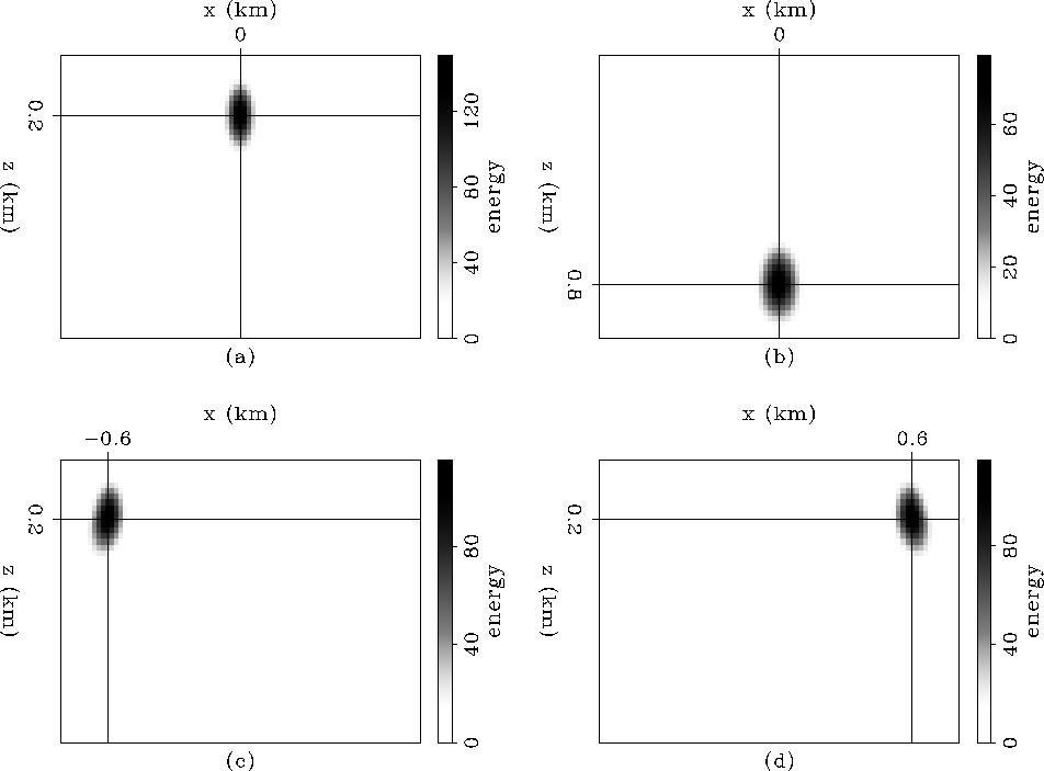
, each line of the Hessian ![]() can be mapped to a grid the size of the model space. Figures and show the Hessian and the envelope of the Hessian at four different fixed points. The Hessian (Figure ) has phase information that can make it difficult to interpret in complex subsurface geometries (see Sigsbee and Marmousi model case), therefore we based our analysis looking at the envelope of the Hessian, (Figure ), which shows clearly the main features of interest.
can be mapped to a grid the size of the model space. Figures and show the Hessian and the envelope of the Hessian at four different fixed points. The Hessian (Figure ) has phase information that can make it difficult to interpret in complex subsurface geometries (see Sigsbee and Marmousi model case), therefore we based our analysis looking at the envelope of the Hessian, (Figure ), which shows clearly the main features of interest.
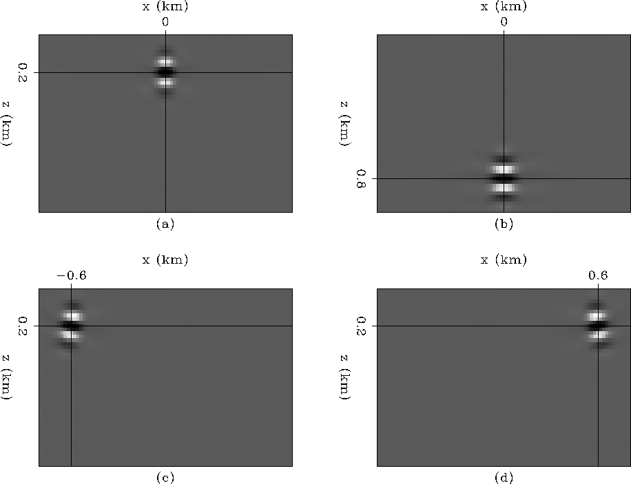 |
Figure a shows point 1, with coordinates ![]() (at the center of the acquisition). Notice the size of the ellipse and the orientation of the principal semi-axis perpendicular to the x axis. Figure b shows point 2, with coordinates
(at the center of the acquisition). Notice the size of the ellipse and the orientation of the principal semi-axis perpendicular to the x axis. Figure b shows point 2, with coordinates ![]() . Notice that the ellipse is bigger than the ellipse corresponding to point 1 (the size of the ellipse depends on the deph and background velocity Chavent and Plessix (1999)), and also that the orientation of the principal semi-axis is perpendicular to the x axis. Figures c and d show points 3 and 4, with coordinates
. Notice that the ellipse is bigger than the ellipse corresponding to point 1 (the size of the ellipse depends on the deph and background velocity Chavent and Plessix (1999)), and also that the orientation of the principal semi-axis is perpendicular to the x axis. Figures c and d show points 3 and 4, with coordinates ![]() and
and ![]() , respectively (opposite sides of the center of the acquisition). Notice the size of the ellipses are the same, but the orientation of the principal semi-axes are tilted in opposite directions. The energy of the ellipses become dimmer than the one in the center, indicating that these points have lower illumination.
, respectively (opposite sides of the center of the acquisition). Notice the size of the ellipses are the same, but the orientation of the principal semi-axes are tilted in opposite directions. The energy of the ellipses become dimmer than the one in the center, indicating that these points have lower illumination.
 |