LSJIMP Review

LSJIMP models the recorded data as the sum of primary reflections and p orders of pegleg multiples from $n_{\rm surf}$ multiple generators. An $i^{\rm th}$-order pegleg splits into i+1 legs. Denoting the primaries $\bold d_0$ and the $k^{\rm th}$ leg of the $i^{\rm th}$ order pegleg from the $m^{\rm th}$ multiple generator $\bold d_{i,k,m}$, the modeled data takes the following form:  

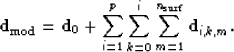$$\bold d_{\rm mod} = \bold d_0 + \sum_{i=1}^p \sum_{k=0}^i \sum_{m=1}^{n_{\rm surf}} \bold d_{i,k,m}.$$ (1)

If we have designed imaging operators that map primaries and multiples to comparable signal events (kinematics and angle-dependent amplitudes), we can write the $\bold d_{i,k,m}$ as linear functions of prestack images. We can similarly denote the modeling operators (adjoint to imaging) for primaries and peglegs as $\bold L_0$ and $\bold L_{i,k,m}$, respectively, and the images of the primaries and peglegs as $\bold m_0$ and $\bold m_{i,k,m}$, respectively. Rewriting equation (1), we have:  

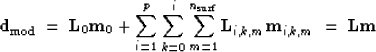$$\bold d_{\rm mod} \; = \; \bold L_0 \bold m_0 + \sum_{i=1}^p... ... surf}} \bold L_{i,k,m} \bold m_{i,k,m} \; = \; \bold L \bold m$$ (2)

The LSJIMP method optimizes the primary and multiple images, $\bold m$, by minimizing the $\ell_2$ norm of the difference between the recorded data, $\bold d$, and the modeled data, $\bold d_{\rm mod}$:  

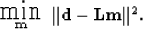$$\mbox{ \raisebox{-1.0ex}{ $\stackrel{\textstyle \mbox{\LARGE... ...tyle \bold m} $} } \; \Vert \bold d - \bold L \bold m \Vert^2.$$ (3)

Minimization (3) is under-determined for most choices of $\bold L_0$ and $\bold L_{i,k,m}$, implying infinitely many solutions. Crosstalk leakage is a symptom of the problem. For instance, $\bold L_0$ maps residual first-order multiple energy in $\bold m_0$ to the position of a first-order multiple in data space. Minimization (3) alone cannot distinguish between crosstalk and signal. Without model regularization, the basic LSJIMP problem is intractable.

Previously Brown (2003b), I devised discriminants between crosstalk and signal, and used them to derive three model regularization operators which choose the set of primary and multiple images which are optimally free of crosstalk. Moreover, these operators exploit signal multiplicity-within and between images-to increase signal fidelity, fill coverage gaps, and combine multiple and primary information. These model regularization operators are the key to the LSJIMP method's novelty.

To solve the regularized LSJIMP problem, we supplement minimization (3) with the three model regularization operators:  

$$\mbox{ \raisebox{-1.0ex}{ $\stackrel{\textstyle \mbox{\LARGE... ...]} \Vert^2 \; + \; \epsilon_3^2 \Vert \bold r_m^{[3]} \Vert^2.$$ (4)

$\bold r_m^{[1]}$, $\bold r_m^{[2]}$, and $\bold r_m^{[3]}$ are the model residuals corresponding to differencing across images, differencing across offset, and crosstalk penalty weighting, respectively. Scalars $\epsilon_1, \epsilon_2,$and $\epsilon_3$ balance the relative weight of the three model residuals with the data residual. I use the conjugate gradient method for minimization (4).

Previously Brown (2003a,c), I outlined an efficient prestack, true relative amplitude imaging scheme for pegleg multiples. We can rewrite $\bold L_{i,k,m}$ as the cascade of a differential geometric spreading correction for multiples ($\bold G_{i,m}$), Snell Resampling to normalize a multiple's AVO to its primary ($\bold S_{i,m}$), HEMNO (Heterogeneous Earth Multiple NMO Operator) to kinematically image split peglegs ($\bold N_{i,k,m}$), and finally, application of the multiple generator's spatially-variant reflection coefficient ($\bold R_{i,k,m}$):  

$$\bold L_{i,k,m} = \bold R_{i,k,m} \bold N_{i,k,m} \bold S_{i,m} \bold G_{i,m}.$$ (5)

The imaging operator for primaries, $\bold L_0$, is simply NMO. The imaged multiples and primaries on the $\bold m_{i,k,m}$ in equation (2) are directly comparable in terms of kinematics and amplitudes. We can exploit this important fact (with model regularization) to discriminate crosstalk from signal, and also to spread information between the images. A true relative amplitude imaging scheme like equation (5) is crucial to fully leverage the multiples in this joint imaging algorithm. Since we apply the operator and its adjoint many times in iterative optimization, computational efficiency is crucial. Because HEMNO images (like NMO) by vertical stretch, equation (5) is fast, memory-conserving, and robust to poorly sampled wavefields, which are the norm with 3-D acquisition. Brown and Guitton (2004) demonstrated that this modeling/imaging approach can accurately model multiples, even in a moderately complex earth.