


Next: Case I. , A*
Up: Eigenvectors for Transverse Isotropy
Previous: Eigenvectors for Transverse Isotropy
If we define the effective compliance matrix for the system as
S* having the matrix elements given in (11), then
the bulk modulus for this system is defined in terms of v1 by
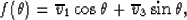
| 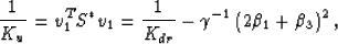 |
(13) |
where the T superscript indicates the transpose, and 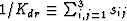 .This is the result usually quoted as Gassmann's equation for the bulk
modulus of the undrained (or confined) anisotropic (VTI) system.
Also, note that in general
.This is the result usually quoted as Gassmann's equation for the bulk
modulus of the undrained (or confined) anisotropic (VTI) system.
Also, note that in general
|  |
(14) |
Thus, even though v1 is not an eigenvector of this system,
it nevertheless plays a fundamental role in the mechanics. Furthermore,
this role is quite well-understood. What is perhaps not so
well-understood then, especially for poroelastic systems, is
the role of v3. Understanding this role will become our main
focus for the remainder of this discussion.
The true eigenvectors of the  subproblem of interest (i.e.,
in the space orthogonal to the four pure shear eigenvectors already
discussed) are necessarily linear combinations of v1 and v3. We can
construct the relevant contracted operator for the
subsystem by considering:
subproblem of interest (i.e.,
in the space orthogonal to the four pure shear eigenvectors already
discussed) are necessarily linear combinations of v1 and v3. We can
construct the relevant contracted operator for the
subsystem by considering:
| 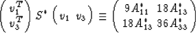 |
(15) |
(in all cases the * superscripts indicate that the pore-fluid
effects are included) and the reduced matrix
|  |
(16) |
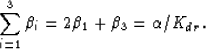
where
| ![\begin{eqnarray}
A^*_{11} = [2(s^*_{11}+s^*_{12}+2s^*_{13})+s^*_{33}]/9, \nonumb...
...A^*_{33} = (s^*_{11}+s^*_{12}-4s^*_{13}+2s^*_{33})/18. \nonumber
\end{eqnarray}](img40.gif) |
|
| (17) |
| |
Providing some understanding of these connections and the implications
for shear modulus dependence on fluid content is one of our goals.
First we remark that A*11 = 1/9Ku, where Ku is again the
undrained (or Gassmann) bulk modulus for the system in (13).
Therefore,
A*11 is proportional to the undrained bulk compliance of this
system. The other two matrix elements cannot be given such simple
interpretations in general. To simplify the analysis we note that, at
least for purposes of modeling, anisotropy of the compliances sij
and the poroelastic coefficients  can be treated
independently.
Anisotropy displayed in the sij's corresponds mostly to the
anisotropy in the solid elastic components of the system, while
anisotropy in the 's corresponds mostly to anisotropy in the
shapes and spatial distribution of the porosity. We will therefore
distinguish these contributions by calling anisotropy appearing in the
sij's the ``hard anisotropy,'' and the anisotropy in the
's will in contrast be called the ``soft anisotropy.''
can be treated
independently.
Anisotropy displayed in the sij's corresponds mostly to the
anisotropy in the solid elastic components of the system, while
anisotropy in the 's corresponds mostly to anisotropy in the
shapes and spatial distribution of the porosity. We will therefore
distinguish these contributions by calling anisotropy appearing in the
sij's the ``hard anisotropy,'' and the anisotropy in the
's will in contrast be called the ``soft anisotropy.''
Now, it is clear (also see the discussion in the Appendix for more
details) that the eigenvectors having unit magnitude
 for this problem
(i.e., for the reduced operator
for this problem
(i.e., for the reduced operator  ) necessarily take the form
|  |
(18) |
where  and
and
 are the normalized eigenvectors.
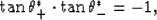
Two solutions for the rotation angle are:
are the normalized eigenvectors.
Two solutions for the rotation angle are:  and
and  , guaranteeing that the
two solutions (the eigenvectors) are orthogonal. It is easily seen
that the eigenvalues are given by
, guaranteeing that the
two solutions (the eigenvectors) are orthogonal. It is easily seen
that the eigenvalues are given by
| ![\begin{eqnarray}
\Lambda^*_\pm = 3\left[A^*_{33} + A^*_{11}/2\pm
\sqrt{(A^*_{33}-A^*_{11}/2)^2 + 2(A^*_{13})^2}\right]
\end{eqnarray}](img49.gif) |
(19) |
and the rotation angles are determined by
| ![\begin{eqnarray}
\tan\theta^*_\pm = {{\Lambda^*_\pm/3 - A^*_{11}}\over{\sqrt{2}A...
...A^*_{33}-A^*_{11}/2)^2 + 2(A^*_{13})^2}\right]/\sqrt{2}A^*_{13}.
\end{eqnarray}](img50.gif) |
(20) |
One part of the rotation angle is due to the drained (fluid free)
``hard anisotropic'' nature of the rock frame material. We will call
this part  . The
remainder is due to the presence of the fluid in the pores, and we will
call this part
. The
remainder is due to the presence of the fluid in the pores, and we will
call this part  for the
``soft anisotropy.'' Using a standard formula for tangents, we have
for the
``soft anisotropy.'' Using a standard formula for tangents, we have
| ![\begin{eqnarray}
\delta\theta_\pm = \tan^{-1}\left[{{\tan\theta^*_\pm
-\tan{\bar...
..._\pm}\over{1 +
\tan\theta^*_\pm \tan{\bar{\theta}}_\pm}}\right].
\end{eqnarray}](img53.gif) |
(21) |
Furthermore, definite formulas for  are found from
(20) by taking
are found from
(20) by taking  (corresponding
to air saturation of the pores).
(corresponding
to air saturation of the pores).
Since
|  |
(22) |
it is sufficient to consider just one of the signs in front of the
radical in (20). The most convenient choice for
analytical purposes turns out to be the minus sign (which corresponds
to the eigenvector with the larger component of pure compression).
Furthermore, it is also clear from the form of (20) that
often the behavior of most interest to us here
occurs for cases when  .
.
In the limit of a nearly isotropic solid frame
(so the ``hard anisotropy'' vanishes
and thus we will also call this the ``quasi-isotropic'' limit), it is
not hard to see that
| 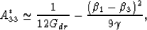 |
(23) |
where Gdr is the drained shear modulus of the
quasi-isotropic solid frame.
Similarly, the remaining coefficient
| 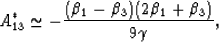 |
(24) |
since all the solid contributions approximately cancel in this limit.
To clarify the situation further, we will enumerate three cases: