COMPUTED EXAMPLES

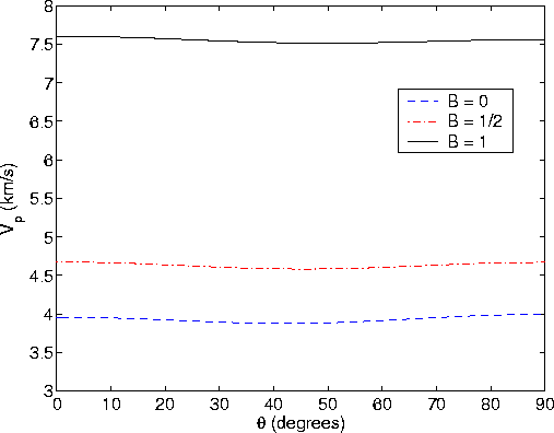
From previous work (Berryman, 2003), we know that large fluctuations in the layer shear moduli are required before significant deviations from Gassmann's quasi-static constant result, thereby showing that the shear modulus dependence on fluid properties can become noticeable. To generate a model that demonstrates these results, again I made use of the same code of V. Grechka as described when presenting Figure 1. But this time I arbitrarily picked just one of the models that seemed to be most interesting for the present purposes. The parameters of this model are displayed in TABLE 1. The results for the various elastic coefficients and Thomsen parameters are displayed in TABLE 2. The results of the calculations for V_p and V_sv are shown in Figures 1 and 2.

The model calculations were simplified in one way: the value of the Biot-Willis parameter was chosen to be a uniform value of $\alpha = 0.8$ in all layers. We could have actually computed a value of $\alpha$ from the other layer parameters, but to do so would require another assumption about the porosity values in each layer. Doing this seemed an exercise of little value because we are just trying to show in a simple way that the formulas given here really do produce the types of results predicted analytically, and also to get a feeling for the magnitude of the effects. Furthermore, if $\alpha$ is a constant, then it is only the product $\alpha B$ that matters. Whatever choice of constant $\alpha \le 1$ is made, it mainly determines the maximum value of the product $\alpha B$ for B in the range [0, 1]. So, for a parameter study, it is only important not to choose too a small value of $\alpha$,which is why the choice $\alpha = 0.8$ was made. This means that the maximum amplification of the bulk modulus due to fluid effects can be as high as a factor of 5 [$= 1/(1-\alpha)$] for the present examples.

TABLE 1. Layer parameters for the three materials in a simple layered medium used to produce the examples in Figures 2 and 3. For this model, $\gamma = 7.882$(indicating strong anisotropy).

$$\mu$$ Constituent K (GPa) z (m/m)

1  9.4541 0.0965 0.477

2 14.7926 4.0290 0.276

3 43.5854 8.7785 0.247

TABLE 2. The VTI elastic coefficients and Thomsen parameters for the materials (see Table 1) used in the computed examples of Figures 2 and 3.

Elastic Parameters Case Case Case

$$B = {{1}\over{2}}$$ and Density B = 0 B = 1

a (GPa) 33.8345 50.3523 132.7003

c (GPa) 33.1948 50.4715 134.2036

f (GPa) 22.2062 38.5857 120.7006

l (GPa)  4.0138  4.0138   4.0138

m (GPa)  6.7777  6.7777   6.7777

G_eff (GPa)  5.2797  5.8841   6.2417

$$\delta$$ -0.0847 -0.0733  -0.0399

$$\epsilon - \delta$$  0.0943  0.0745   0.0343

$$\gamma$$  0.3443  0.3443   0.3443

$$\rho$$  2120.0  2310.0  2320.0

We took the porosity to be $\phi = 0.2$, and the overall density to be $\rho = (1-\phi)\rho_s + \phi S \rho_l$, where $\rho_s = 2650.0$ kg/m³, S is liquid saturation ($0 \le S \le 1$), and $\rho_l = 1000.0$ kg/m³. Then, three cases were considered: (1) Gas saturation S=0 and B=0, which is also the drained case, assuming that the effect of the saturating gas on the moduli is negligible. (2) Partial liquid saturation S = 0.95 and $B = {{1}\over{2}}$ [which is intended to model a case of partial liquid saturation], intermediate between the other two cases. For smaller values of liquid saturation, the effect of the liquid might not be noticeable, since the gas-liquid mixture when homogeneously mixed will act much like the pure gas in compression, although the density effect will still be present. When the liquid fills most of the pore-space, and the gas occupies less than about $3\%$ of the entire volume of the rock, the gas starts to become disconnected, and we expect the effect of the liquid to start becoming more noticeable, and therefore we choose $B = {{1}\over{2}}$ to be representative of this case. And, finally, (3) full liquid saturation S = 1 and B=1, which is also the fully undrained case. We assume for the purposes of this example that a fully saturating liquid has the maximum possible stiffening effect on the locally microhomogeneous, isotropic, poroelastic medium.

 

vpnew
Figure 2 Compressional wave speed V_p as a function of angle $\theta$ from the vertical. Two curves shown correspond to choices of Skempton's coefficient B = 0 for the drained case (dashed line) and B=1 for the undrained case (solid line). The case $B = {{1}\over{2}}$ (dot-dash line) is used to model partial saturation conditions as described in the text. The Biot-Willis parameter was chosen to be $\alpha = 0.8$, constant in all layers.

 

vsnew
Figure 3 Vertically polarized shear wave speed V_sv as a function of angle $\theta$ from the vertical. Two curves shown correspond to choices of Skempton's coefficient B = 0 for the drained case (dashed line) and B=1 for the undrained case (solid). The case $B = {{1}\over{2}}$ (dot-dash line) is used to model partial saturation conditions as described in the text. The Biot-Willis parameter was chosen to be $\alpha = 0.8$, constant in all layers.

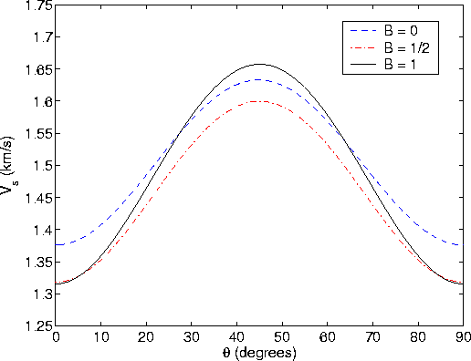The results shown in Figures 2 and 3 are in complete qualitative and quantitative agreement with the analytical predictions described, as expected.