Ray-coordinate triplication

The phase-ray extrapolation examples discussed so far have intentionally avoided triplicating wavefields. However, wavefield triplications are commonly observed in seismic data, especially in areas of complex geology where the phase-ray extrapolation technique shows most potential. In this formulation, the ray coordinate system is computed from previous wavefield steps; hence, the underlying basis will begin to triplicate immediately after the wavefield does. Thus, a contingency plan must exist to prevent numerical instabilities associated with coordinate triplication.

Wavefield triplication naturally occurs when a propagating wavefield is focused by lateral velocity variation acting as an optic lens. One canonical example is a Gaussian-shaped slow velocity anomaly, where continued wavefields exhibit a characteristic bow-tie signature beneath the anomaly. Numerical instabilities occur when calculating the ray coordinate system in the vicinity of the bow-tie because neighboring rays overlap while following their respective branches of the bow-tie. At the crossing point, the Jacobian in equation (8) is identically zero leading to infinite values of wavenumber $k_\tau$ in equation (6). Infinite wavenumbers, of course, are not realizable in practice and are only a theoretical artifice of the wavefield being multivalued at that point. Accordingly, instabilities with ray coordinate triplication may be rectified through an appropriate accounting for the wavefield's multivalued nature during numerical calculations.

One way to deal with multivalued functions is to treat the individual branches of the triplication bow-tie as independent wavefield components that should be held incommunicado. This idea, borrowed from ideas in the mathematical field of complex analysis Cohn (1967), is illustrated in Figure 8.

 

branch Figure 8 Cartoon of our methodology of splitting different branches of a triplication. Left: Triplication where the 3 branches lie on the same plane; Right: Same triplication as in left panel, but with each branch residing on a separate plane. Our method is to effectively restrict communication between branches when calculating derivatives and other associated quantities.

Isolating triplication branches requires computing the locations of wavefield triplications from crossing ray segments in the rayfield. In 2-D, crossing ray segments may be identified by modeling the segments as infinite lines, computing their intersection point, and testing whether this location falls within the area bounded by the ray segments. Where this test reveals a crossing point (or branch point), the rayfield has triplicated and should be cut into individual branches. Jacobian coordinate and other related functions that require the computation of derivatives, can be then be calculated on their respective branches (i.e. on one of the three planes in Figure 8). For locations not on branch cuts, centered finite-difference stencils may be used; however, at branch-cut locations appropriate left- and right-sided derivatives are required. Importantly, the locations of branch cuts are kept for all subsequent computations. Finally, we acknowledge that this treatment of rayfield triplication is cursory and remains a topic of ongoing research. However, similarities between our proposed method for handling coordinate triplications and the standard branch cut technique of complex analysis should provide us with a powerful set of tools for further development.

The canonical example of a slow Gaussian-shaped velocity anomaly is presented in Figure 9.

 

Gauss.ps
Figure 9 Canonical example of a slow Gaussian velocity perturbation. Left: model with background velocity 2000m/s on which is superposed a slow Gaussian of -50$\%$ of the background velocity, and the 10Hz coordinate system. Middle: 10Hz monochromatic image. Right: broadband (0.1-30Hz) wavefield calculated using a stationary 10Hz ray coordinate system.

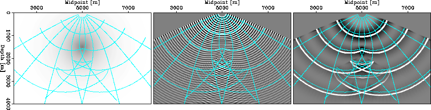The velocity model used in this example is presented in the left panel, and consists of a slow Gaussian anomaly of maximum -50$\%$perturbation of the 2000m/s background velocity. The 10Hz phase-ray coordinate system is also overlain. The middle panel shows the 10Hz wavefield. The hatched pattern in the lower center of the figure is created by the superposition of the phases of the two competing triplication branches (as discussed in Shragge and Biondi (2003)). The right panel presents the broadband result (0.1-30Hz) computed on a stationary 10Hz phase-ray coordinate system. In the lower part of the figure, the signature bow-ties of the triplicating wavefield are evident. The slight undulations on the centered part of the bow-tie, though, should not be present. Our conjecture is that these are an artifact of coordinate system interpolation.