


To illustrate the application and results of NW seismic alignment, we present three examples. The first is alignment of events in synthetic P-wave and S-wave zero-offset sections. The second is flattening of events in a common image gather (CIG) from a marine 2D seismic line. In the final case we attempt to align a real P- and S-wave section.
For the first example, two synthetic zero-offset seismic sections (Figure 1) were generated by 2D acoustic Kirchhoff modeling. The data is moderately complex, containing low and steep dips, diffractions, and a buried focus. The subsurface reflector geometry is identical in each case. The S-wave section (Figure 1b) was modeled using the P-wave velocities and a VS-VP ratio that varied both laterally and with depth. This means a spatially-variant, nonlinear stretch is needed to align the sections. The alignment algorithm works here in a pairwise fashion on each trace pair that has the same trace number in each section. Every alignment is calculated independently, so there is no error propagation in this case.
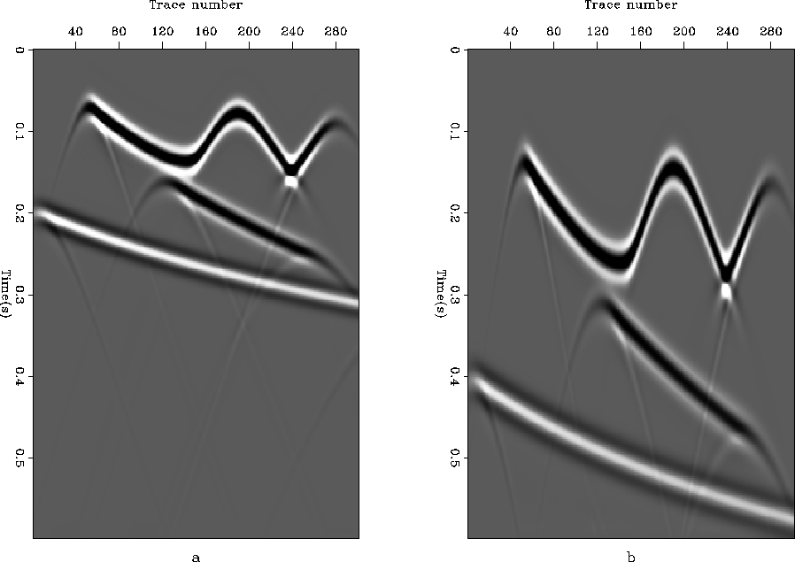 |

The alignment result (Figure 2) represents the P-wave section
after application of nonlinear stretch coefficients.
We could just as easily have aligned the S-wave section to the P-wave data.
The gap penalties for this example are (p,q)=(0.0,0.1) and ![]() .
Comparison of the S-wave section (Figure 1)
with the alignment section demonstrates the accuracy and sensitivity of
this method.
Considering the complexity of the input data, we feel the alignment is
of excellent quality.
.
Comparison of the S-wave section (Figure 1)
with the alignment section demonstrates the accuracy and sensitivity of
this method.
Considering the complexity of the input data, we feel the alignment is
of excellent quality.
 |
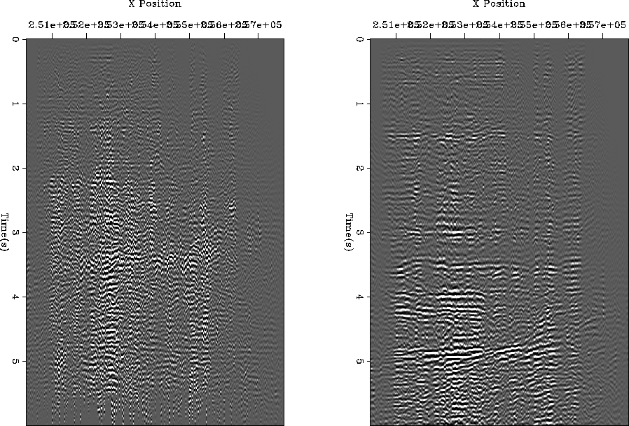
For a second example, we chose a common reflection point gather from a 2D marine data set (left panel of Figure 3). This collection of traces forms an common image gather in the angle domain Prucha et al. (1999); Sava and Fomel (2000) after phase-shift plus-interpolation (PSPI) migration Gazdag and Sguazzero (1985). Note that we see some residual moveout in the CIG. The number of events, low-slope residual moveout, and lateral variations make this a significant alignment problem. The goal here is to align events in the gather with the first (zero-angle) trace. Constructing the aligned model in this case is far more complex than the procedure necessary for independent pairwise trace alignments. The effect of aligning trace two to trace one affects the alignment of traces three and two, etc.
In our view, there are three potential ways around this connectivity.
The first is to do the alignments sequentially. Align trace n-1 to
trace n, then align both n and n-1 to n-2, and repeat the procedure
until all traces are aligned. This procedure can be effective but
is prone to error propagation.
The second is to recognize that all possible pairs of traces can be aligned
to each other and setup an inverse problem that takes all possible
alignments into account. This would probably lead to the best
solution but how best to relate the different combinations isn't obvious
and the computational cost is significantly increased (we now have
to compute and account for ![]() comparisons).
comparisons).
We chose a third approach to multi-trace alignment involving a linear operator that performs sequential shifting. The idea is to begin at an initial trace (for example, the near offset) and to work outward toward the final trace (far offset). As each trace pair is aligned, these alignment coefficients (ACs) are applied to all remaining traces. In this way, an intermediate trace receives many partial alignments, and one last alignment from its nearest neighbor which itself has been modified several times. The algorithm can be summarized as follows:
     for trace i from 1 to (n-1) {
         for trace j from (i+1) to n {
              modify trace j using ACs between traces i and (i+1)
         }
     }
This method evolved from extensive testing of alternative approaches, each of which introduced serious error propagation problems.
In this case, single application of the algorithm was not sufficient. In order to
obtain a reasonable solution, a larger gap penalty (p,q) = (0.1,0.5) was
found to be necessary, along with ![]() as in the CMP test.
The resulting section still had residual moveout. As a result we
reversed the output of the first alignment along the time axis and used this
as input to a second run of the alignment procedure.
Total compute time on a workstation-class machine was 25 seconds.
The right panel of
Figure 3 shows the result after the two-pass alignment.
The flattening is not perfect, but the events are much better aligned than before
while maintaining the same amplitude versus angle (AVA) characteristics.
as in the CMP test.
The resulting section still had residual moveout. As a result we
reversed the output of the first alignment along the time axis and used this
as input to a second run of the alignment procedure.
Total compute time on a workstation-class machine was 25 seconds.
The right panel of
Figure 3 shows the result after the two-pass alignment.
The flattening is not perfect, but the events are much better aligned than before
while maintaining the same amplitude versus angle (AVA) characteristics.
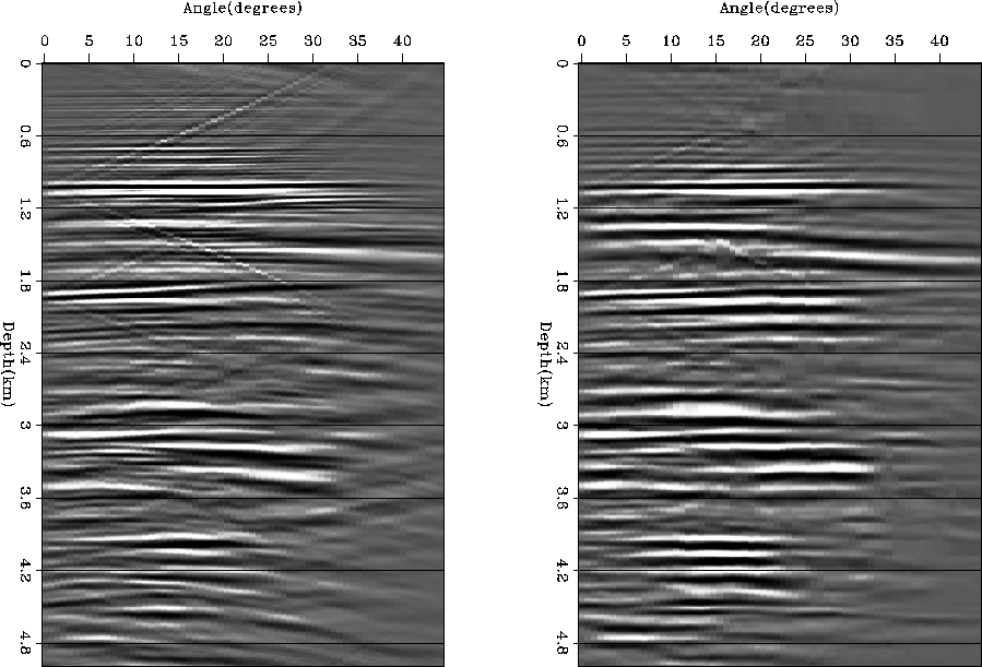 |
For the final example, we attempted to align a PP and PS stacked section from the Alba field in the North Sea. Figure 4 shows the PP and PS section before alignment. This problem poses significant additional problems compared to the synthetic used in the first example. We are dealing with much higher frequency data than the first example and have many more events. The left panel of Figure 5 shows the output of the alignment procedure. Note the jumps in the sections, and the gaps at certain CMP locations. The first problem is an inherent property of the algorithm. The penalty we can impose for jumps is limited. The second problem is because we are performing a series of independent alignments. The result of the previous alignment has no affect on the current alignment. As a result we get the inconsistencies seen in the image.
 |
 |