 |
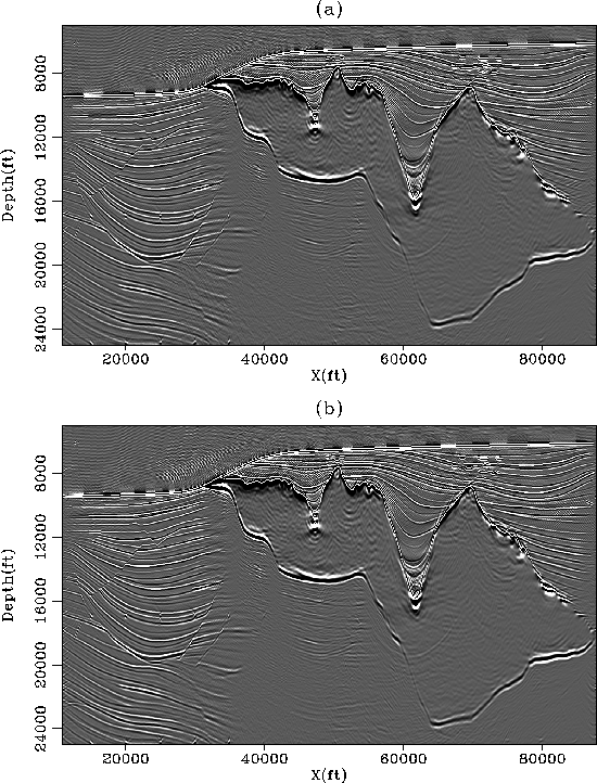
Figure 7 Two constant offset sections (h=1125 ft) after multiple attenuation with the Spitz approximation using (a) 2D and (b) 3D filters.
![[*]](http://sepwww.stanford.edu/latex2html/movie.gif)
Now I assume that only a model of the multiples is known. The Spitz approximation in equation (12) shows how the PEFs for the signal can be estimated. Because deconvolution with non-stationary filters is unstable, the noise PEFs is convolved with the data and the signal PEFs is then estimated from the convolution result.
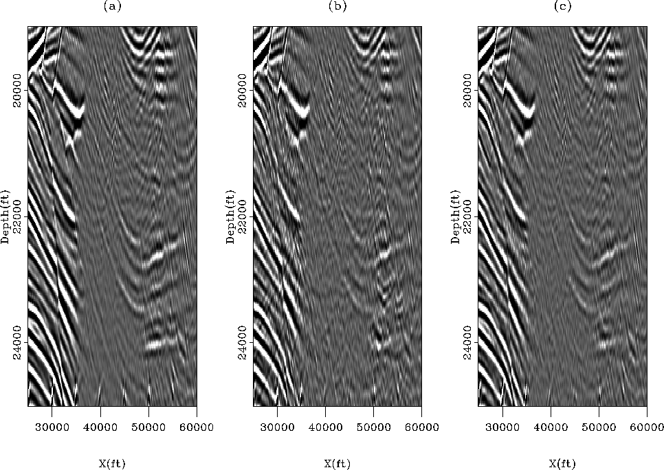
The primaries are recovered with 2D and 3D filters. Figure 7 displays two constant offset sections after multiple attenuation with 2D and 3D PEFs. 3D PEFs give by far the best results and attenuate multiples very well. After migration, we see again in Figure 8 that the 3D PEFs better attenuate the multiples. A close-up in Figure 9 demonstrates in more detail how the two results with 2D or 3D filters differ below the salt. Events are more continuous and better preserved with 3D filters. Comparing with the true reflectors in Figure 9a, important primaries are attenuated with both 2D and 3D filters. This is particularly true where the signal is the weakest (between midpoint positions 35 and 50 kft).
This important observations could not have been made before migration in the prestack domain because the primaries are much weaker than the surface-related multiples below the salt. This illustrates the point that for complex geology, the quality of a multiple removal technique should be assessed in the image space as often as possible. For this analysis to be successful, accurate velocity and migration algorithm must be provided as well. Finally, the fact that some primaries are attenuated in Figure 9 should motivate us in devising improved strategies for building better noise and signal models.
 |
![[*]](http://sepwww.stanford.edu/latex2html/movie.gif)
 |
![[*]](http://sepwww.stanford.edu/latex2html/movie.gif)
 |
![[*]](http://sepwww.stanford.edu/latex2html/movie.gif)