 |
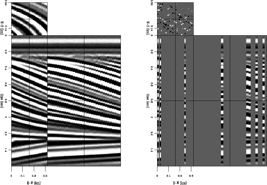
Figure 2 Left: 32x32-trace subset of the quarter dome model. The subset was selected to be less sensitive to spatial aliasing than the steeper-dipping portions of the model. Right: Missing data test, with 100 known traces and 924 missing traces.
![[*]](http://sepwww.stanford.edu/latex2html/cross_ref_motif.gif) . Only
100 out of 1024 input traces are assumed known, for a decimation rate of over 90
percent. The dip estimated by my method will then be used to interpolate the
missing trace locations by solving the system (7)-(9).
. Only
100 out of 1024 input traces are assumed known, for a decimation rate of over 90
percent. The dip estimated by my method will then be used to interpolate the
missing trace locations by solving the system (7)-(9).
 |
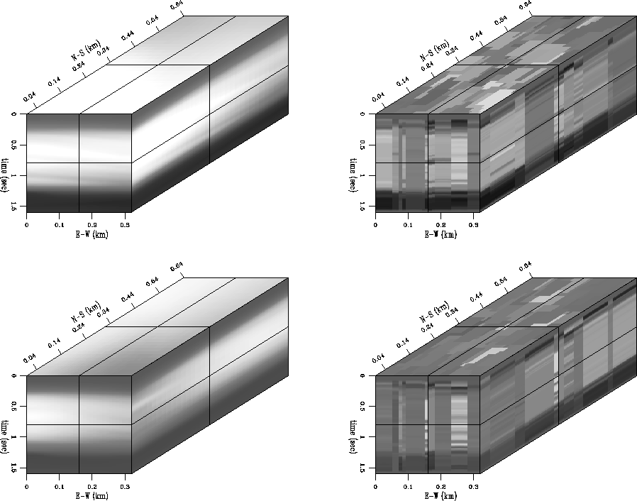
The left panels of Figure ![[*]](http://sepwww.stanford.edu/latex2html/cross_ref_motif.gif) show the quarter dome model's
``known'' dip, which was computed using a variant of Fomel's
2002 dip estimation method. The right panels show the
dip estimated from the irregularly-sampled traces shown in Figure
show the quarter dome model's
``known'' dip, which was computed using a variant of Fomel's
2002 dip estimation method. The right panels show the
dip estimated from the irregularly-sampled traces shown in Figure
![[*]](http://sepwww.stanford.edu/latex2html/cross_ref_motif.gif) , using the method described herein. To smooth the dip
estimates between master trace locations, I use an expanding-window smoothing
program.
, using the method described herein. To smooth the dip
estimates between master trace locations, I use an expanding-window smoothing
program.
While the dip estimates are decidedly imperfect, they nontheless do contain the general trends seen in the known dip fields. Particularly note the unconformity deep in the section. We see that in the more steeply-dipping parts of the section, my method tends to underestimate the reflector dip. Since the decimation is severe, spatial aliasing may arise, even if the dips are not severe, because my method measures dip directly between two arbitrary traces. Claerbout's puck method is known to be sensitive to spatial aliasing. Fomel (2002) discusses ways to de-sensitize dip estimation with respect to spatial aliasing.
 |
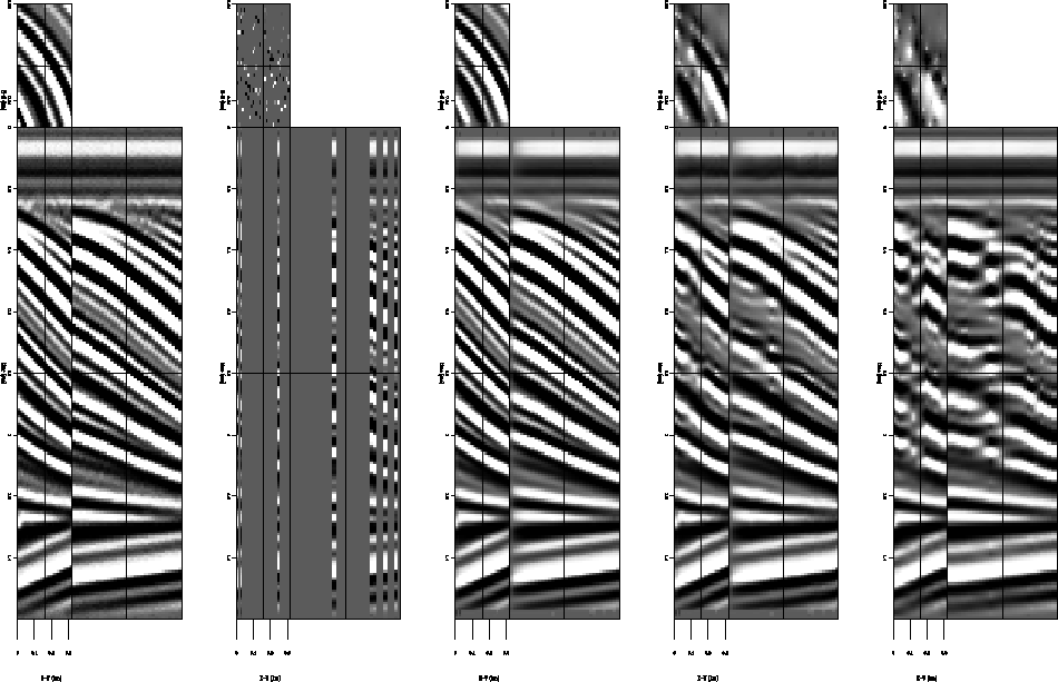
Figure ![[*]](http://sepwww.stanford.edu/latex2html/cross_ref_motif.gif) compares the result of using: a) the known dip,
b) the dip estimated from the irregular data, and c) zero dip in solving
equations (7)-(9) for an infilled model. We see that
in spite of the imperfections of the dip estimated from the irregular data, that
it definitely leads to a better inverse interpolation result that the zero dip
result, which just smoothes laterally. All results were computed using 20
iterations of a linear conjugate gradient solver.
compares the result of using: a) the known dip,
b) the dip estimated from the irregular data, and c) zero dip in solving
equations (7)-(9) for an infilled model. We see that
in spite of the imperfections of the dip estimated from the irregular data, that
it definitely leads to a better inverse interpolation result that the zero dip
result, which just smoothes laterally. All results were computed using 20
iterations of a linear conjugate gradient solver.
 |