Locating regions for potential discontinuity locations

The coherency evaluation explained in the previous section will produce a coherency cube for a 3D seismic image. In the coherency cube, the discontinuity information is expressed as a distribution of the event continuity with numerical values ranging from 1 to 0 corresponding to the semblance of events at each location. A conventional interpretation process takes another step to map the discontuinity surfaces with the help of various visualization tools.

It is obvious that the discontinuity surfaces will be located somewhere in the region where the coherency value is lower than its neighbor. The shape of the discontinuity surface will be similar to the shape of the region that has lower coherency values than others. Therefore, a rough 3D shape of the discontinuity surfaces can be obtained in a binary image form obtained by thresholding the coherency cube as follows:

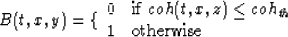$$B(t,x,y) = \{ \begin{array} {cl} 0& \mbox{if } coh(t,x,z) \leq coh_{th}\\ 1& \mbox{otherwise } \\ \end{array}$$ (3)

where the thresholding value, coh_th, is determined empirically with a trial and error approach. The image needs to be histogram-equalized before thresholding, which requires the image to be quantized. I quantized the coherency value by rounding it to the nearest hundredth value, then applied histogram equalization to make sure each coherency value is distributed evenly so that the thresholding value change effects for the binary image shape appropriately. 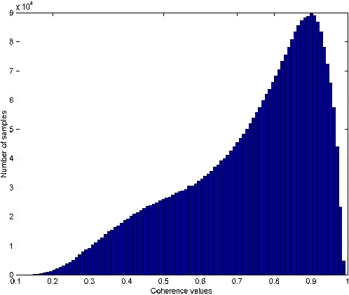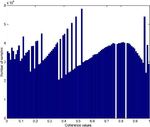Figures 5 and 6 show the histogram of quantized coherency values and its result after histogram equalization, respectively. 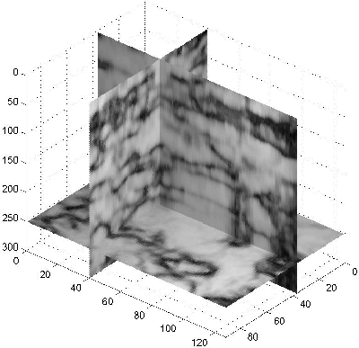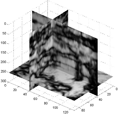The effect of the quantization and the equalization on the image can be seen in Figures 7 and 8. By increasing the contrast, the unclear low coherency region in Figure 7 becomes clear in Figure 8.

 

histogram
Figure 5 Histogram of the quantized coherency cube.

 

histogrameq
Figure 6 Histogram of the quantized coherency cube after histogram equalization.

 

coh-quantize
Figure 7 The coherency cube after quantization applied with 0.01 quantization level.

 

coh-heq
Figure 8 The coherency cube after the histogram equalization applied.

 

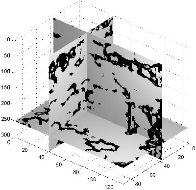
binary20
Figure 9 Binary image obtained by selecting points whose values are less than 0.2 from the histogram equalized coherency cube.

 

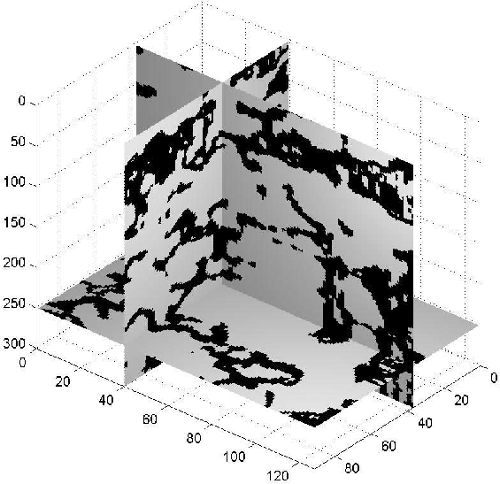
binary-30
Figure 10 Binary image obtained by selecting points whose values are less than 0.3 from the histogram equalized coherency cube.

 

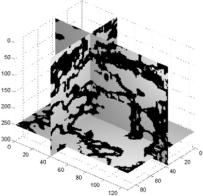
binary-40
Figure 11 Binary image obtained by selecting points whose values are less than 0.4 from the histogram equalized coherency cube.

The effects on the binary image shape with respect to different thresholding values are shown in Figures 9 through 11. Figure 9, 10 and 11 are images obtained by thresholding Figure 8 with 0.2, 0.3, and 0.4, respectively. From those figures, we can see that increasing the thresholding value makes the binary image shape get thicker, as expected.