Grid Shifting

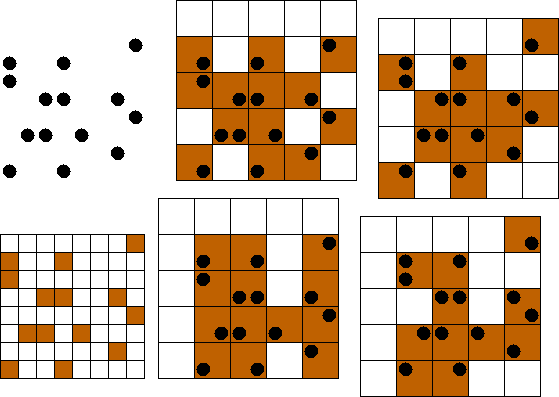
Instead of simply taking multiple scales of data ($\bf{d_i}$), multiple different grid locations can be used for each scale, as there is freedom in how they are chosen. For the case of a grid twice as coarse as the original fine grid, there would be 4 possible grid locations for a 2D case, shown in Figure 1. This number is inversely proportional to the size of the bins, and increases exponentially with dimension. However, in the case of irregular traces, there is no point in shifting the grid along the time axis, as the number of equations would be unaffected.

 

shift
Figure 1 Shifting grids, clockwise from lower left: original fine-scale data; data points extracted from that fine grid; and four different grid orientations for a single coarser scale. Dots signify data, colored bins contain data, and white bins are empty.

In the case of a non-stationary PEF, extra bookkeeping is required, as the different grid locations will correspond to different regions of the non-stationary PEF. This does make using these extra versions of the data more expensive, as the weight $\bf{W}$ and sub-sampler $\bf{P}$ are not the same at one scale and need to be recomputed.