Dipping planes

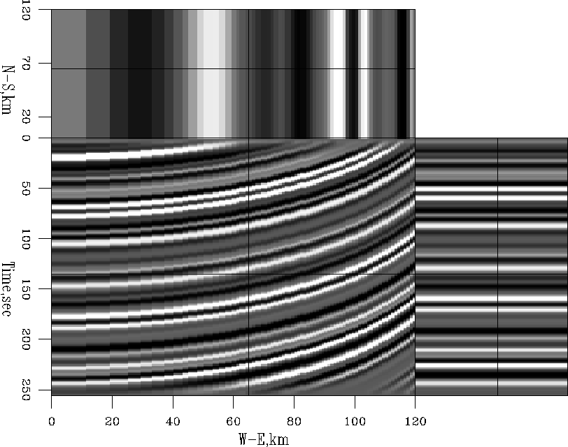
The 3D synthetic data set in Figure 1 consists of a single synthetic seismic trace that is replicated and delayed so that the dip in both the x and y directions is unity. Running a dip estimator as in equation (1) will ideally result in dips of one in each direction.

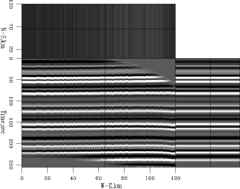
The results of the flattening method of the data in Figure 1 are shown in Figure 2. Notice that the dipping planes are now flat and that the time slice on top is all one gray tone, indicating that it is flat.

 

ski_jmp
Figure 3 Test case 2. Curved horizons.

 

ski_jmp.3Dflat
Figure 4 Result of flattening data in Figure 3.

 

chev
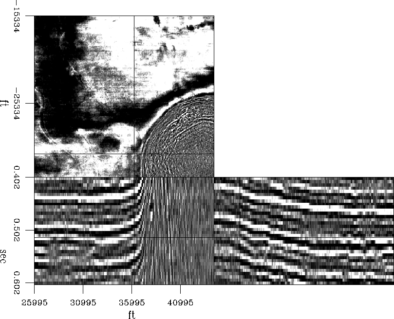
Figure 5 Test case 3. Chevron Gulf of Mexico data.

 

chev.3Dflat
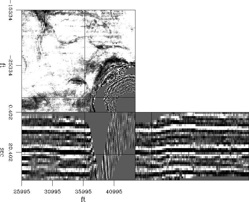
Figure 6 Result of flattening data in Figure 5.

 

chev_ts
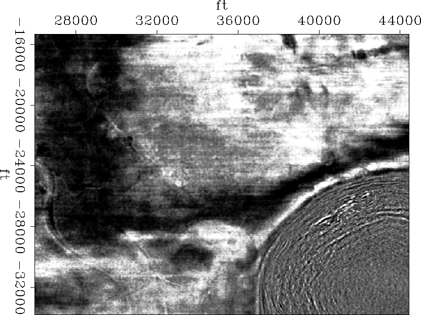
Figure 7 Time slice from Unflattened Chevron Gulf of Mexico data.

 

chev.3Dflat_ts
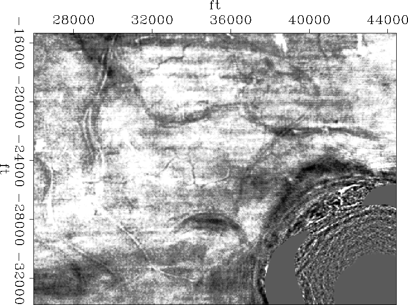
Figure 8 Time slice from Flattened Chevron Gulf of Mexico data.