The scatterplot between AVA attributes and shale volume

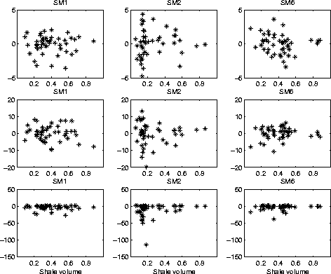
We extracted AVA attributes (intercept, gradient, and their product) at three well locations: CMPX=3.875km for well A, 5.375km for well B and 4.575km for well C. The well log has much higher vertical resolution than seismic data, so, in order to correlate the AVA attributes and log data at same depth, we used sinc function to interpolate the log data. I applied the same depth window that ranges from 3.12 km to 3.57 km for the three wells and scatterploted AVA attributes and shale volume. Figure 4 show the result. We can't see obvious correlation between AVA attributes and shale volume in this figure, but we can tell that the shale volume in the depth window along well B has a much lower value than other two wells.

 

scatter
Figure 4 Scatterplot between AVA attributes and shale volume. From left to right, the column is for well A, B and C, respectively; from up to bottom, the y-axis is intercept, gradient and their product respectively. The x-axis is shale volume for all of them.

Theoretically, AVA attributes will correlate better with impedance rather than shale volume. Unfortunately, we didn't have density log for well A and B. We scatterploted velocity from sonic log and AVA attributes for all three wells. We didn't see any positive caused high AVA uncertainty here.