Experiment

To explore the feasibility of this idea, we used the solar data set that has been seen in several previous reports. The frequency content of this data shows two distinct modes as seen in Figure 1. The previous results generated by autocorrelation processing Rickett and Claerbout (1999) used a low-cut version of the data that removes the energy below 2 mHz.

 

spec Figure 1 Frequency content of the passive solar seismic data set. Data are sampled in Kilo-seconds yielding milli-Hertz frequencies.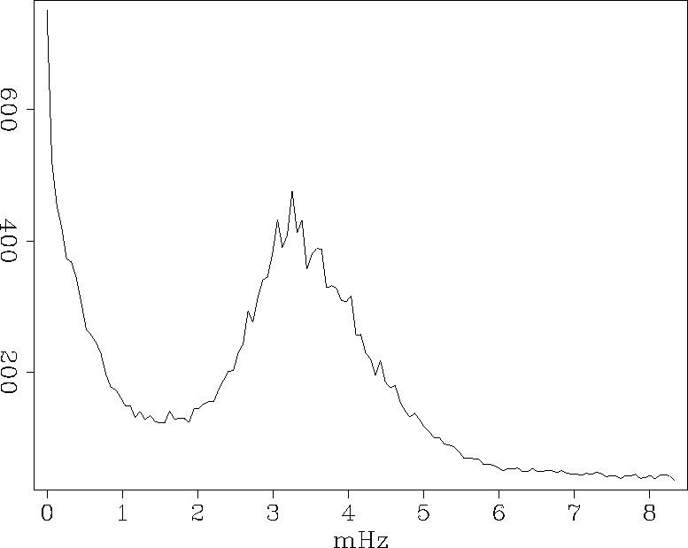

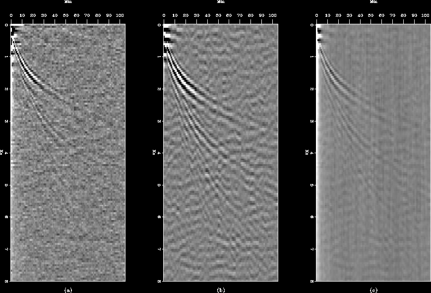
Figure 2 is a comparison of three different inputs to the autocorrelation processing algorithm. The right panel uses the raw data. The center panel uses a low-cut version of the data. The left panel is the output after 1-dimensional deconvolution. Unfortunately, a small amount of DC noise has survived the deconvolution process. Because the solar data is not quite as stationary as had been hoped, estimating the PEF on too small an area resulted in an output spectrum that is not white in all locations. Some color left in the frequency content of the result would seem acceptable; however, the low-frequency contribution to the result presents a problem in the auto-correlation processing.

 

three
Figure 2 Left panel is autocorrelation after deconvolution. Center panel is processing after low-cut filter. Right panel is produced using the raw data.

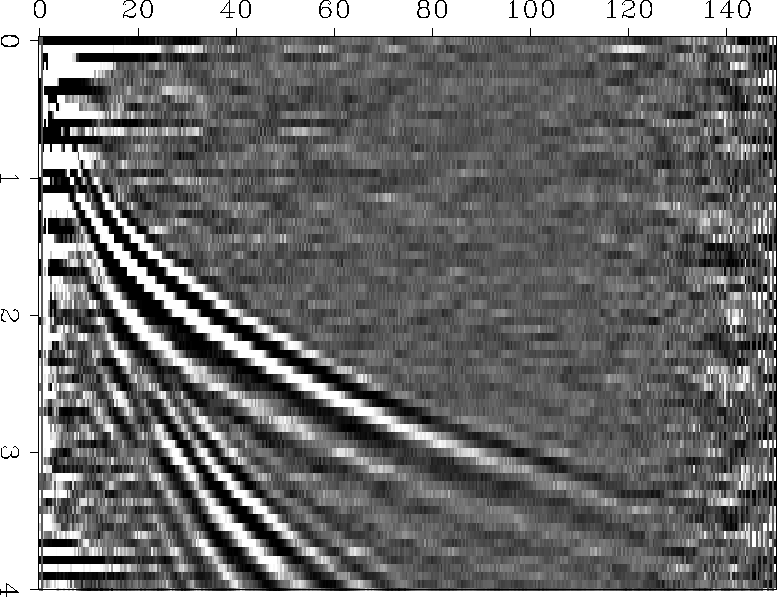
To better combat this near-D.C. component of the data, all of the traces were passed through a 1D gradient operator. Having thus removed the low-frequency component of the data, the PEF estimation and convolution process was performed again followed by auto-correlation processing. Figure 3 shows the result of this processing scheme. The result is better focused, crisper and more pleasing than the results shown in Rickett and Claerbout (1999) generated by low-cut filtering and auto-correlation processing.

 

newevent Figure 3 After 1D gradient, deconvolution, and auto-correlation processing the solar passive seismic data may reveal faint new events on this in-line section. Look carefully for 3 dark linear events: from (0Mm,0ks), (10Mm,0ks), and (40Mm,0Ks). The velocity of these events is approximately 50,000 m/s.

The first in-line section of the result of this processing chain is shown in Figure 3 and seems to show three faint events that have not been previously identified. Unfortunately, further evidence to corroborate them as real events have not been fruitful. Perpendicular sections do not reveal similar events. Time slices do not show circular horizon intersections. Finally, an azimuthal stack around the central trace was calculated. Figure 4 shows this result with no indication of the earlier events.

 

radstack
Figure 4 Radial stack of previous data to see if the ``events'' might stack into reality. No further evidence of the events.