Limiting the scanning range

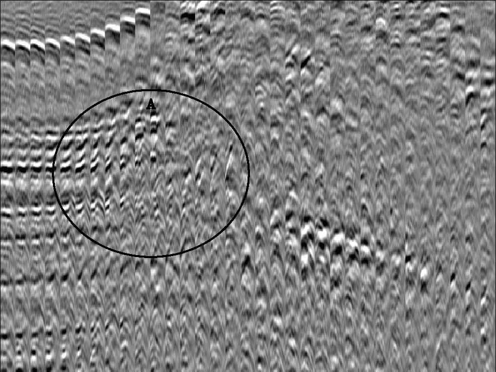
In Clapp (2001a), I outlined a procedure for selecting points for back projection. The goal was to find points with high dip coherence and semblance at a minimum distance from each other. This methodology can run into problems for events whose moveout doesn't correspond to primary events or whose moveout is not adequately defined by calculating vertical semblance. For example, the common reflection point (CRP) gathers in Figure 1 shows every fifth gather along the left edge of a salt body. Note the coherent but ``hockey stick'' like shapes within the `A' oval. These can be caused by small velocity errors Biondi and Symes (2002) but measuring just vertical moveout would indicate much larger errors. Clapp (2002) shows one way to address the latter concern.

 

gathers
Figure 1 Every 5th gather to the left edge of a salt body. Note the coherent, ``hockey stick'' behavior within `A'.

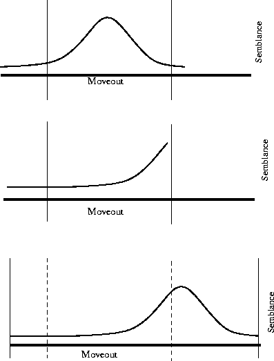
Simply limiting the range of acceptable moveouts that we search isn't a sufficient solution because the maximum often will be at the extreme scan range. A simple methodology to minimize the effect of unreasonable moveouts is to scan over a large range of acceptable moveouts and only accept points whose maximum fall within a smaller range (see Figure 2). With this methodology, spurious moveouts can be identified and ignored. When dealing with internal multiples or events whose moveout is close to acceptable, failure can still result.

 

limited Figure 2 The top figure shows an example of a good point. The maximum is reasonable and within the scanning region indicated by the solid vertical lines. The second plot shows the problematic situation. The moveout is unreasonable and its maximum is outside the scanning range. We can avoid using the unrealistic moveout by scanning over moveouts between the solid lines but only selecting points whose maximum is within the dashed lines, bottom panel.

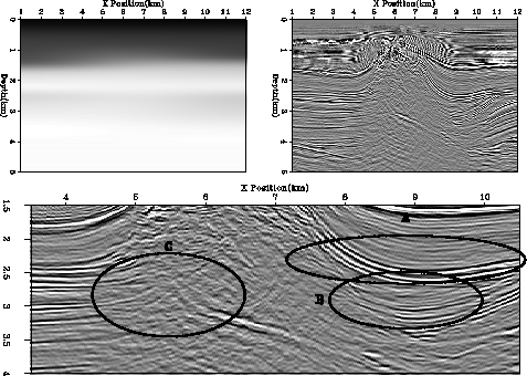
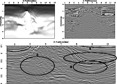
To show the benefits of this methodology, I applied it to a complex 2-D dataset. Figure 3 shows an initial velocity model and migrated image of a 2-D line from a 3-D dataset donated by Total Fina Elf. Figure 4 shows the updated velocity model and migrated image without limiting the scan range. Note the extreme velocity along the edge of the salt. The resulting image is less coherent than the initial image, especially in the ovals indicated by `A', `B', and `C'. 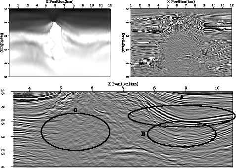Figure 5 shows the result of limiting the range of acceptable moveouts. Note how the velocity along the edge is more reasonable. We see a strong salt bottom reflection at `A', better definition of the valley at `B', and more coherent events leading up to the salt edge at `C'.

 

combo.vel0
Figure 3 The starting model and migration of a 2-D line from a 3-D North Sea dataset. The top-left panel shows the velocity model (white indicates large velocities) and the top-right panel shows the migrated image using this velocity. The bottom panel shows a zoomed area around the salt body. Note the salt bottom,`A'; the valley structure at `B'; and over the salt under-hang at `C'.

 

combo.vel1.bad
Figure 4 Data after one non-linear iteration. The top-left panel shows the velocity model and the top-right panel shows the migrated image using this velocity. The bottom panel shows a zoomed area around the salt body. Note the salt bottom,`A'; the valley structure at `B'; and under the salt over-hang at `C'.

 

combo.vel1.l2
Figure 5 Data after one non-linear iteration with limited semblance search window. The top-left panel shows the velocity model and the top-right panel shows the migrated image using this velocity. The bottom panel shows a zoomed area around the salt body. Note the salt bottom,`A'; the valley structure at `B'; and under the salt over-hang at `C'. Note the improvements compared to Figure 4.