EXAMPLES

To test the methodology we started with a simple synthetic Normal Moveout (NMO) gather with some random noise (Figure 2). We selected two traces some distance apart (the first and tenth trace) and applied the algorithm. The two traces can be seen in the left part of Figure 3. Note the time-variant alignment error.

 

nmo.gather Figure 2 A synthetic shot gather. The first and tenth trace were selected to test the algorithm.

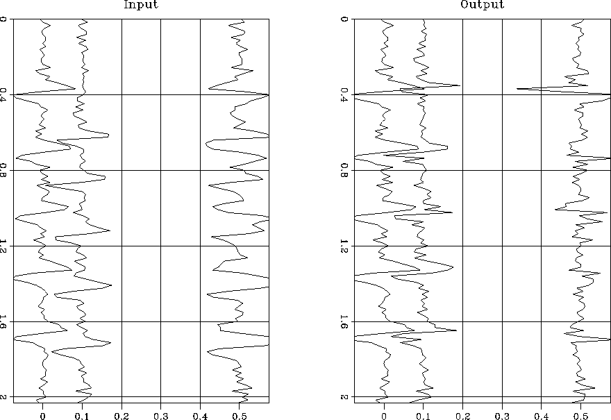
Figure 4 shows the similarity (left) and score (right) matrices. The black lines in the similarity matrix represent low scores and correspond to the events in the data, they only disappear (or match) when encountering another wavelet. The score matrix shows exactly what we expect to see. A slightly non-diagonal maximum (except for edge effects at low times corresponding to a lack of coherent events). Figure 3 shows the input (left) and output (right) along with their corresponding differences. The output is much better aligned and the overall differences reduced. The difference trace is a proxy for guaging the quality of alignment, but the goal is not to drive this difference to zero. The algorithm keys on strong events whose alignment may result in sizable differences at other levels. This is a significant departure from Martinson and Hopper (1992) who minimize a difference measure to determine alignment.

 

nmo.in-out Figure 3 The left plot shows the two input traces and the right plot the traces after alignment. The third trace in each display shows the difference.

 

nmo.score-sim
Figure 4 The right plot is the score matrix using first two traces from Figure 2 and the left panel is the similarity matrix. Axes labels refer to time sample numbers (not seconds).

For a second test we chose a common reflection point (CRP) gather from a 2-D marine dataset (Figure 5). The gather is an angle gather Prucha et al. (1999); Sava and Fomel (2000) after phase-shift plus-interpolation (PSPI) migration Gazdag and Sguazzero (1985). Note that we still see some residual moveout in the angle gather. The left panel of Figure 7 shows the input two traces (third and sixteenth).

After running the algorithm we obtained the score and similarity matrices seen in Figure 6. Note how the structure of the similarity matrix to the previous example (Figure 4). The score matrix and the corresponding maximum has the shape that we would anticipate. It is generally diagonal with some deviations. The output two traces appear to be better aligned (the right panel of Figure 7), but the difference isn't as reduced as we would hope. Our belief is this caused by a poor stretching algorithm.

 

big.gather Figure 5 The CRP gather used for trace alignment. The third and 16th trace were used.

 

big.score-sim
Figure 6 The right plot is the score matrix using two traces from a CRP gather and the left panel is the similarity matrix. Axes labels refer to time sample numbers (not seconds).

 

big.in-out Figure 7 The left plot shows the two input traces and the right plot the traces after alignment in the window from three to four seconds. The third trace in each display shows the difference.