EXAMPLE

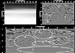
To test the methodology I chose a 2-D line from a 3-D North Sea dataset. Figure 6 shows

• the initial velocity model (top-left panel),
• the initial migration (top-right), and
• a zoomed in portion of the model with three regions highlighted for future comparisons (bottom).

 

combo.vel0
Figure 6 The initial model and migration. The top-left panel shows the velocity model and the top-right panel shows the migrated image using this velocity. The bottom panel shows a blow up around the salt body. `A' - `E' will be used later in the text for comparison.

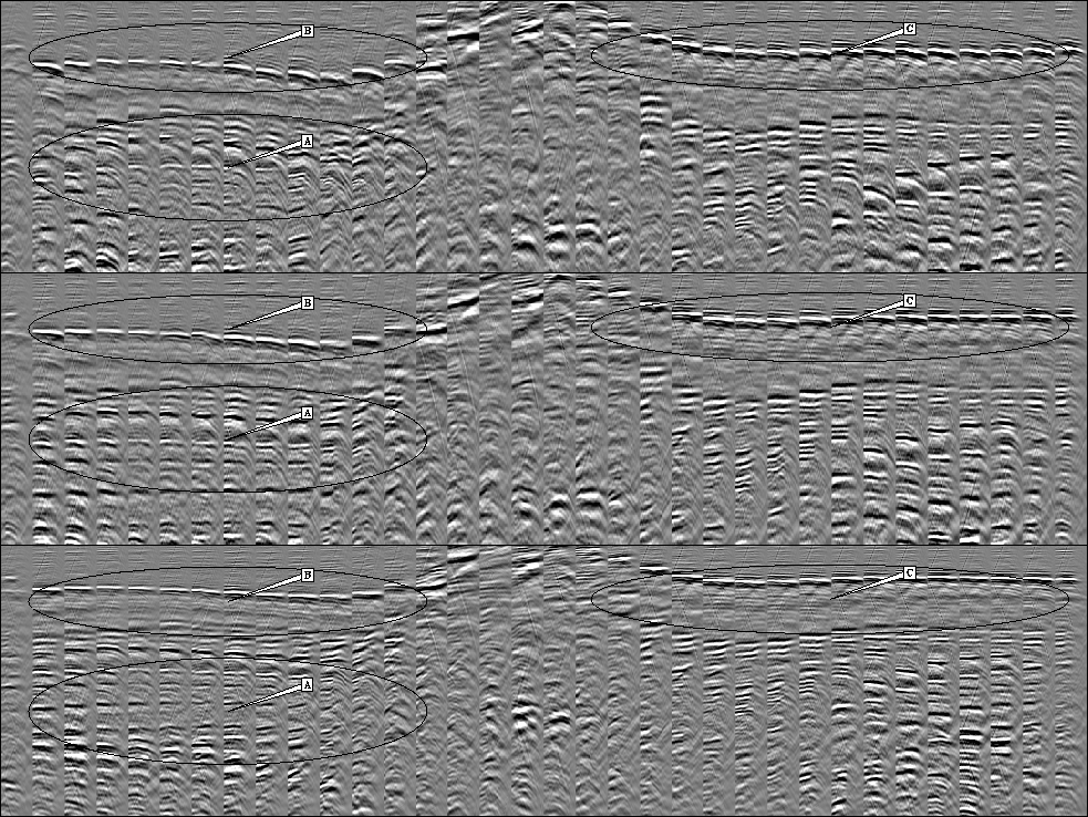
I performed one non-linear iteration of tomography using three different approaches. The top panel of Figure 7 shows the result of using vertical moveout as the basis for determining the time errors. The center panel is again the result of using vertical moveout for the time error calculation with additional constraints on what points are used for back projection and limiting the effect of bad moveouts Clapp (2002). The bottom panel is the result of using residual migration.

The area signified with `A' shows the problems with using all of the data (top panel). Note how the gathers have tremendous, inconsistent curvature. When we discount this information (center panel) we get more reasonable gathers. Using residual migration to estimate $\bf \Delta t$we can get the same, or better, gathers without throwing away a portion of the data. The problem with throwing away a portion of the data can been at `C' and especially `B'. We threw away the information that would help us flatten the reflector in order to avoid the problems seen in the top panel. Smply using vertical moveout analysis, it takes several non-linear iterations to achieve the same level of flatness at `A' and `B' that is seen with the first non-linear iteration using a residual migration measure.

 

gathers.iter1
Figure 7 Each panel represents every 15th CRP gather between 1 and 4 km after one non-linear iteration of tomography. The top panel is the result of performing tomography calculating $\bf \Delta t$ using vertical moveout. The center panel is using vertical moveout discounting data with significant moveout. The bottom panel shows the result of using residual migration as the basis of the $\bf \Delta t$ calculation. Note the improved flatness of the CRP gathers from top to bottom.

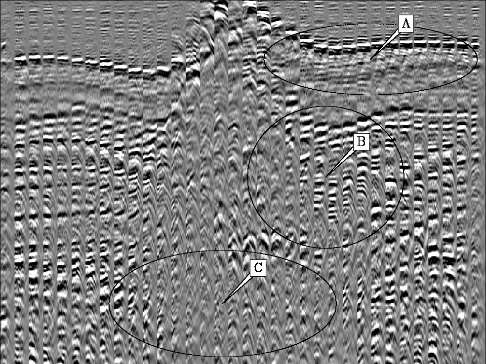
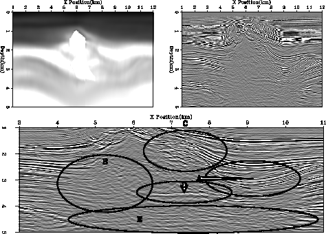
Figure 8 shows every 15th CRP gather after five non-linear iterations. Note how the moveout in reflector at `A' is virtually flat. Within valley structure, `B', there is little remaining residual moveout. The most interesting location is `C' where we are begining to see coherent events under the salt. Figure 9 shows the resulting velocity and image after five non-linear iterations. The salt top reflection is now clean. Note how the valley structure at `A' is well imaged. At `B' we can follow reflectors all the way to what appears to be the salt edge. On the top-left portion of the salt, `C', we have gone from a jumbled mess (Figure 6) to being able to clearly follow reflectors. At `D' we see a consitant, strong amplitude, salt bottom reflection. Finally, at `E' we are begining to see strong events under the salt. Further improvement requires going to 3-D.

 

gathers.final
Figure 8 Every 15th CRP gather after five non-linear iterations. Note the flat gathers at `A' and `B' and the forming of coherent moveout below the salt at `C'.

 

combo.final
Figure 9 Data after five non-linear iterations of tomography with residual migration based moveout analysis. The top-left panel shows the velocity model and the top-right panel shows the migrated image using this velocity. The bottom panel shows a blow up around the salt body. Note how the valley structure at `A' is well imaged. At `B' we can follow reflectors all the way to what appears to be the salt edge. On the top-left portion of the salt, `C', we have gone from a jumbled mesh (Figure 6) to being able to clearly follow reflectors. At `D' we see a consistent, strong amplitude, salt bottom reflection. Finally, at `E' we are begining to see the forming of fairly strong events under the salt.

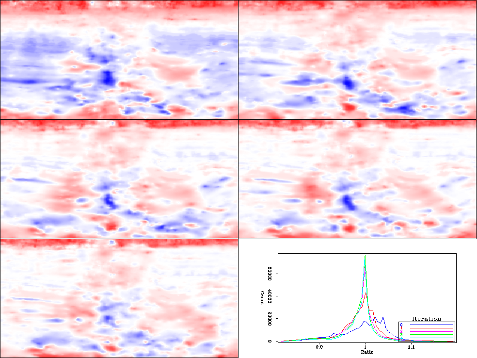
Another way to evaluate image improvement is to look at the $\gamma$ values after successive iterations. Figure 10 show the $\gamma$ values after zero to four iterations (left to right, top to bottom). The figure demonstrates that as we progress in iteration the $\gamma$ value tends towards 1, indicating that the problem is converging.

 

ratios
Figure 10 The residual moveout measure as a function of non-linear iteration. The top-left is the initial moveout, the top-right after one iteration, etc. The bottom-right panel shows a histogram for each of the $\gamma$ maps. Note how the points cluster towards 1 as we progress in iteration. Note how the ratio tends towards 1 (no-moveout, white) as we progress. The red stripe on top is due to the severe early mute. The offset to angle transform has an edge effect that causes the data to curve up. As a result the best flatness is obtained with a very low $\gamma$ value. These values are ignored in the inversion.