IMAGING PROBLEM

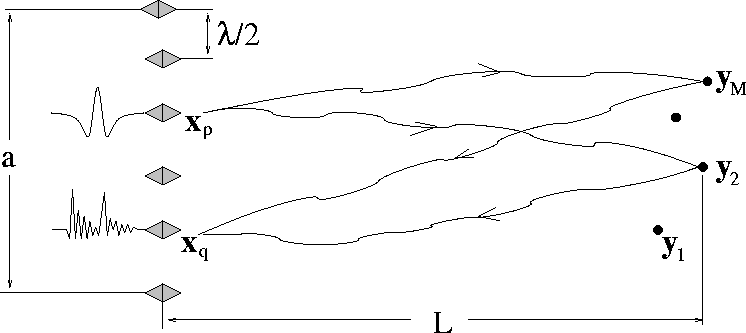
Our analysis assumes that the array has N transducers located at spatial positions ${\bf x}_p$, for $p = 1,\ldots, N$. (See Figure 1.) When used in active mode, the array probes the unknown acoustic medium containing M small scatterers by emitting pulses and recording the time traces of the back-scattered echos. We call the resulting data set the multistatic array response (or transfer) matrix  

$$P(t)=\left(P_{pq}(t)\right),$$ (1)

where p and q both range over all the array elements. For our simulations, we consider a linear array where two adjacent point transducers are a distance $\lambda/2$ apart, with $\lambda$ being the carrier (central) wavelength of the probing pulses. Such an arrangement ensures that the collection of transducers behaves like an array having aperture $a = (N-1) \lambda/2$ and not like separate entities, while keeping the interference among the transducers at a minimum (Steinberg, 1983). Our goal is to detect and then localize all M of the targets in the random medium, if possible.

 

gen_setup
Figure 1 Array probing of a randomly inhomogeneous medium containing M small scatterers.

For the numerical examples considered here, we will treat ultrasonic imaging problems. Our simulations assume that $\lambda \le \ell << a = (N-1)\lambda/2 << L$,where $\lambda$ is the central wavelength, $\ell$ is a characteristic length scale of the inhomogeneity (like a correlation length), a is the array aperture, and L is the approximate distance to the targets from the array. This is the regime where multipathing, or multiple scattering, is significant even when the standard deviation of sound speed fluctuations is only a few percent. Values used in the codes are $\lambda = 0.5$mm, a = 2.5mm, and a background wave speed of c₀ = 1.5km/s. More details concerning the simulations may be found in Borcea et al. (2002).

Typical array processing methods assume that the targets are far away from the array and, therefore, they look like points. Similarly, the propagation medium is assumed homogeneous and so the observed wavefronts scattered by the targets look like plane waves at the array. Array noise has usually been treated as due either to diffuse sources of white noise coming simultaneously from all directions, or to isolated ``noise'' having the same types of source characteristics as the targets of interest. But in random media with significant multiple scattering, the resulting ``noise'' cannot be successfully treated in these traditional ways.

Real-space time-reversal processing of the array response data involves an iterative procedure: sending a signal, recording and storing the scattered return signal, time-reversing and then rebroadcasting the stored signal, with subsequent repetitions. This procedure amounts to using the power method for finding the singular vector of the data matrix having the largest singular value. Alternatively, when the full response/transfer matrix has been measured for a multistatic active array, the resulting data matrix can be analyzed directly by Singular Value Decomposition (SVD) to determine not only the singular vector having the largest singular value, but all singular vectors and singular values -- simultaneously (Prada and Fink, 1994; Prada et al., 1996; Mordant et al., 1999).

Imaging is always done using a fictitious medium for the simulated backpropagation that produces these images since the real medium is not known. Its large-scale features could be estimated from other information, such as geological data obtained by seismic methods. For example, migration methods (Claerbout, 1976; Aki and Richards, 1980; Bleistein et al., 2001) can be used, where very large arrays -- much larger than those we contemplate using here -- are required. However, the small-scale random inhomogeneities are not known and cannot be effectively estimated, so the simplest thing to do is ignore them when imaging, and use methods that are statistically stable and therefore insensitive to the exact character of these small inhomogeneities.