DOUBLE-POROSITY THOUGHT EXPERIMENT

  

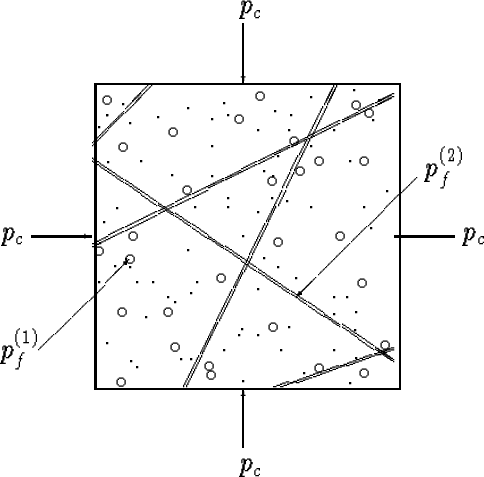
Figure 2: A composite porous medium is composed of two distinct types of porous solid (1,2). In the model illustrated here and treated in the text, the two types of materials are well-bonded but themselves have very different porosity types, one being a storage porosity (type-1) and the other (type-2) being a transport porosity (and therefore fracture-like, or tube-like as illustrated in cross-section in this diagram).

Several of the main results obtained previously can be derived in a more elegant fashion by using a new self-similar (uniform expansion) thought experiment. The basic idea we are going to introduce here is analogous to, but nevertheless distinct from, other thought experiments used in thermoelasticity by Cribb (1968) and in single-porosity poroelasticity by Berryman and Milton (1991) and Berryman and Pride (1998). Cribb's method provided an independent and simpler derivation of Levin's (1967) results on thermoelastic expansion coefficients. The present results also provide an independent and simpler derivation of results obtained recently by Berryman and Pride (2002) for the double-porosity coefficients. Related methods in micromechanics are sometimes called ``the method of uniform fields'' by some authors (Dvorak and Benveniste, 1997).

We have already shown that a₁₁ = 1/K^*. We will now show how to determine the remaining five constants in the case of a binary composite system, such as that illustrated in Figure micropic. The components of the system are themselves porous materials 1 and 2, but each is assumed to be what we call a ``Gassmann material'' satisfying [in analogy to equation (all)]  

$$\left(\begin{array} {c} \delta e^{(1)} - \delta\zeta^{(1)}/... ...c} - \delta p_c^{(1)} - \delta p_f^{(1)} \end{array}\right)$$ (24)

for material 1 and a similar expression for material 2. The new constants appearing on the right are the drained bulk modulus K⁽¹⁾ of material 1, the corresponding Biot-Willis parameter $\alpha^{(1)}$, and the Skempton coefficient B⁽¹⁾. The volume fraction v⁽¹⁾ appears here to correct for the difference between a global fluid content and the corresponding local variable for material 1. The main special characteristic of a Gassmann porous material is that it is composed of only one type of solid constituent, so it is ``microhomogeneous'' in its solid component, and in addition the porosity is randomly, but fairly uniformly, distributed so there is a well-defined constant porosity $\phi^{(1)}$ associated with material 1, etc.

For our new thought experiment, we ask the question: Is it possible to find combinations of $\delta p_c = \delta p_c^{(1)} = \delta p_c^{(2)}$,$\delta p_f^{(1)}$, and $\delta p_f^{(2)}$ such that the expansion or contraction of the system is spatially uniform or self-similar? This is the same as asking if we can find uniform confining pressure $\delta p_c$, and pore-fluid pressures $\delta p_f^{(1)}$ and $\delta p_f^{(2)}$, such that  

$$\delta e = \delta e^{(1)} = \delta e^{(2)}.$$ (25)

If these conditions can all be met simultaneously, then results for system constants can be obtained purely algebraically without ever having to solve the equilibrium equations for nonconstant stress and strain. We have initially set $\delta p_c = \delta p_c^{(1)} = \delta p_c^{(2)}$, as the condition of uniform confining pressure is clearly necessary for this self-similar thought experiment to achieve a valid solution of the equilibrium equations.

So, the first condition to be considered is the equality of the strains of the two constituents:  

$$\delta e^{(1)} = -{{1}\over{K^{(1)}}}(\delta p_c - \alpha^{(... ...}\over{K^{(2)}}}(\delta p_c - \alpha^{(2)} \delta p_f^{(2)}).$$ (26)

If this condition can be satisfied, then the two constituents are expanding or contracting at the same rate and it is clear that self-similarity will prevail. If we imagine that $\delta p_c$ and $\delta p_f^{(1)}$ have been chosen, then we only need to choose an appropriate value of $\delta p_f^{(2)}$, so that (e1e2) is satisfied. This requires that  

$$\delta p_f^{(2)} = \delta p_f^{(2)}(\delta p_c,\delta p_f^{(... ...pha^{(1)}K^{(2)}}\over{\alpha^{(2)}K^{(1)}}}\delta p_f^{(1)},$$ (27)

which shows that, except for some very special choices of the material parameters (such as $\alpha^{(2)} = 0$), $\delta p_f^{(2)}$ can in fact always be chosen so the uniform expansion takes place. (We are not considering long-term effects here. Clearly, if the pressures are left to themselves, they will tend to equilibrate over time so that $\delta p_f^{(1)} = \delta p_f^{(2)}$.We are considering only the ``instantaneous'' behavior of the material permitted by our system of equations and finding what internal consistency of this system of equations implies must be true.)

Using formula (pf2), we can now eliminate $\delta p_f^{(2)}$ from the remaining equality so that  

$$\delta e = -\left[a_{11}\delta p_c + a_{12}\delta p_f^{(1)} ... ...}\over{K^{(1)}}}(\delta p_c - \alpha^{(1)} \delta p_f^{(1)}),$$ (28)

where $\delta p_f^{(2)}(\delta p_c,\delta p_f^{(1)})$ is given by (pf2). Making the substitution and then noting that $\delta p_c$ and $\delta p_f^{(1)}$ were chosen independently and arbitrarily, we see that the resulting coefficients of these two variables must each vanish. The equations we obtain in this way are  

$$a_{11} + a_{13}(1-K^{(2)}/K^{(1)})/\alpha^{(2)} = 1/K^{(1)}$$ (29)

and  

$$a_{12} + a_{13}(\alpha^{(1)}K^{(2)}/\alpha^{(2)}K^{(1)}) = -\alpha^{(1)}/K^{(1)}.$$ (30)

Since a₁₁ is known, equation (fora13) can be solved directly for a₁₃, giving  

$$a_{13} = - {{\alpha^{(2)}}\over{K^{(2)}}}{{1-K^{(1)}/K^*}\over{1-K^{(1)}/K^{(2)}}}$$ (31)

Similarly, since a₁₃ is now known, substituting into (fora12) gives  

$$a_{12} = - {{\alpha^{(1)}}\over{K^{(1)}}}{{1-K^{(2)}/K^*}\over{1-K^{(2)}/K^{(1)}}}.$$ (32)

Thus, three of the six coefficients have been determined.

To evaluate the remaining three coefficients, we must consider what happens to the fluid increments during the same self-similar expansion thought experiment. We will treat only material 1, but the equations for material 2 are completely analogous. >From the preceding equations, it follows that  

$$\delta\zeta^{(1)} = a_{12}\delta p_c + a_{22} \delta p_f^{(1... ...)}\delta p_c + (\alpha^{(1)}/B^{(1)})\delta p_f^{(1)}\right].$$ (33)

Again substituting for $\delta p_f^{(2)}(\delta p_c,\delta p_f^{(1)})$ from (pf2) and noting once more that the resulting equation contains arbitrary values of $\delta p_c$ and $\delta p_f^{(1)}$, so that the coefficients of these terms must vanish separately, gives two equations  

$$a_{12} + a_{23}(1-K^{(2)}/K^{(1)})/\alpha^{(2)} = - \alpha^{(1)}v^{(1)}/K^{(1)},$$ (34)

and  

$$a_{22} + a_{23}\left(\alpha^{(1)}K^{(2)}/\alpha^{(2)}K^{(1)}\right) = \alpha^{(1)}v^{(1)}/B^{(1)}K^{(1)}.$$ (35)

Solving these equations in sequence as before, we obtain  

$$a_{23} = {{K^{(1)}K^{(2)}\alpha^{(1)}\alpha^{(2)}}\over{(K^{... ...{(1)}}} + {{v^{(2)}}\over{K^{(2)}}} - {{1}\over{K^*}}\right],$$ (36)

and  

$$a_{22} = {{v^{(1)}\alpha^{(1)}}\over{B^{(1)}K^{(1)}}} - \lef... ...{(1)}}} + {{v^{(2)}}\over{K^{(2)}}} - {{1}\over{K^*}}\right].$$ (37)

Performing the corresponding calculation for $\delta\zeta^{(2)}$ produces formulas for a₃₂ and a₃₃. Since the formula in (xa23) is already symmetric in the component indices, the formula for a₃₂ provides nothing new. The formula for a₃₃ is easily seen to be identical in form to a₂₂, but with the 1 and 2 indices interchanged everywhere.

This completes the derivation of all five of the needed coefficients of double porosity for the two constituent model.

These results can now be used to show how the constituent properties K, $\alpha$, B average at the macrolevel for a two-constituent composite. We find

$$\begin{eqnarray} \alpha &=& - {{a_{12}+a_{13}}\over{a_{11}}} \nonumber\ &=& {{\a... ...(K^*-K^{(2)})+\alpha^{(2)}(K^{(1)}-K^*)}\over{K^{(1)}-K^{(2)}}}, \end{eqnarray}$$

and

$$\begin{eqnarray} {{1}\over{B}} &=& - {{a_{22}+2a_{23}+a_{33}}\over{a_{12}+a_{13}... ...}}} + {{v^{(2)}}\over{K^{(2)}}} - {{1}\over{K^*}}\right]\right). \end{eqnarray}$$

It should also be clear that parts of the preceding analysis generalize easily to the multi-porosity problem. We discuss some of these remaining issues in the final section.