Possible solutions

One possible solution would be to estimate a 2D PEF using multi-scale PEF estimation Curry and Brown (2001). Another possibility would be to estimate both a 2D PEF and the missing data at the same time in a similar approach to equation 3 from Claerbout (1999) but instead of estimating the PEF everywhere, throw out all fitting equations where the leading 1 of the PEF lands on unknown data. If you were to throw out all fitting equations where any coefficient of the PEF lands on unknown data, there would not be enough fitting equations to actually calculate the PEF. To estimate the PEF ($\bf a$) on a model ($\bf y$), we start with an initial model convolved with an initial filter ($\bf{Ay}$) and perturb them with $\Delta \bf y$ and $\Delta \bf a$. In equation 4 we add the residual weight, $\bf W$, to throw out fitting equations where the first coefficient of $\bf a$ lands on missing data. The free-mask matrix for missing data is denoted $\bold J$ and that for the PEF is $\bold K$. 

$$\bold 0 \quad\approx\quad \left[ \begin{array} {cc} \bol... ...d y \\ \Delta \bold a \end{array} \right] + \bold A \bold y$$ (3)

 

$$\bold 0 \quad\approx\quad \bold W \left[ \left[ \begin{ar... ...\Delta \bold a \end{array} \right] + \bold A \bold y \right]$$ (4)

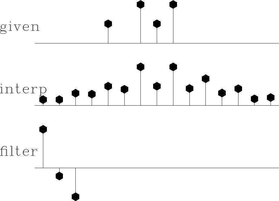
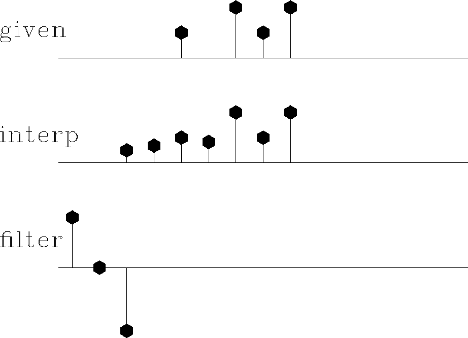
In Claerbout (1999), Figure 13 is generated by estimating both the missing data and unknown filter at the same time. I added a data-space weight as above and got the results in Figure 14. Notice it almost calculates the same filter. It does not completely fill in the missing data because we threw out many fitting equations.

 

misif90 Figure 13 Top is known data. Middle includes the interpolated values. Bottom is the filter with the leftmost point constrained to be unity and other points chosen to minimize output power.

 

misif90_2 Figure 14 Top is known data. Middle includes the interpolated values. Bottom is the filter with the leftmost point constrained to be unity and other points chosen to minimize output power but only throwing out fitting equations where the leftmost point lands on unknown data.

I have tested this only on simple 1D models, not yet on the Madagascar data. For the Madagascar data, the initial filter ($\bf a$) may be the Laplacian.