Forward and Inverse NMO

The NMO correction time for the small offset-spread approximation is given by the well-known hyperbolic equation Yilmaz (1987):

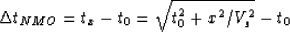$$\Delta t_{NMO}=t_x-t_0=\sqrt{t_0^2+x^2/V_s^2}-t_0$$ (8)

where x is the trace offset, t_x is the two-way travel time at offset x, t₀ is the two-way travel time at zero offset (normal incidence trace) and V_s is the stacking velocity. Clearly, for a given trace different samples will have different NMO correction times even if the velocity is constant. Shallow events on the farthest trace with the slowest velocity have the maximum NMO-correction time whereas deep events on the near traces with the fastest velocity will have the minimum NMO-correction time. It is also important to note that in general some fractional sample interpolation will be required since we cannot expect the values of $\Delta t_{NMO}$ to be integer multiples of the sampling interval.

In order to apply the non-stationary filtering algorithm we need to recast the NMO equation as an all-pass non-stationary filter that will simply shift each sample by the given value of $\Delta t_{NMO}$. This can easily be achieved in the frequency domain by a linear phase shift with slope proportional to the value of $\Delta t_{NMO}$. In principle, any value of $\Delta t_{NMO}$ can be handled, so no fractional interpolation is required. For the sake of efficiency, however, it is convenient to precompute a given number of $\Delta t_{NMO}$ values. The accuracy of the implicit fractional interpolation is determined by the number of precomputed $\Delta t_{NMO}$ values and so can be controlled as an input parameter. Clearly, this parameter controls the trade-off between accuracy and speed of computation.