Next: AVA analysis
Up: Clapp: Effect of velocity
Previous: Clapp: Effect of velocity
The way I formulate my tomography fitting goals requires
some deviation from the generic multi-realization form.
My tomography fitting goals are fully described in Clapp (2001a).
Generally,
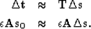
I relate change in slowness  ,to change in travel time
  by a linear operator
  The tomography operator is constructed by linearizing around an
initial slowness model
The tomography operator is constructed by linearizing around an
initial slowness model  . I regularize the slowness
  rather than change in slowness and obtain the fitting goals,
|  |
(4) |
| |
The calculation of  is the same procedure as
shown in equation (3). The only difference
is now we initiate
is the same procedure as
shown in equation (3). The only difference
is now we initiate  with both our
random noise component
with both our
random noise component  and
and  .A cororarly approach for data uncertainty is discussed in Appendix A.
Results
To test the methodology I decided to start with
a structurally simple 2-D line from a land dataset from Columbia
provided by Ecopetrol. Figure 1 shows the
estimated velocity for the data. Note how it is generally
v(z) with some deviation, especially in the lower portion of the image. Figure 2 shows
the result of performing split-step phase shift migration and
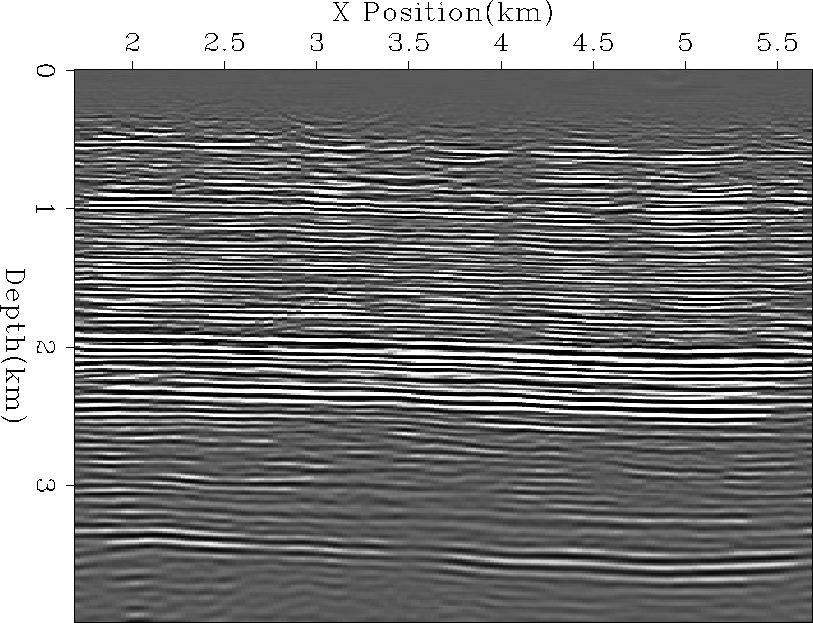
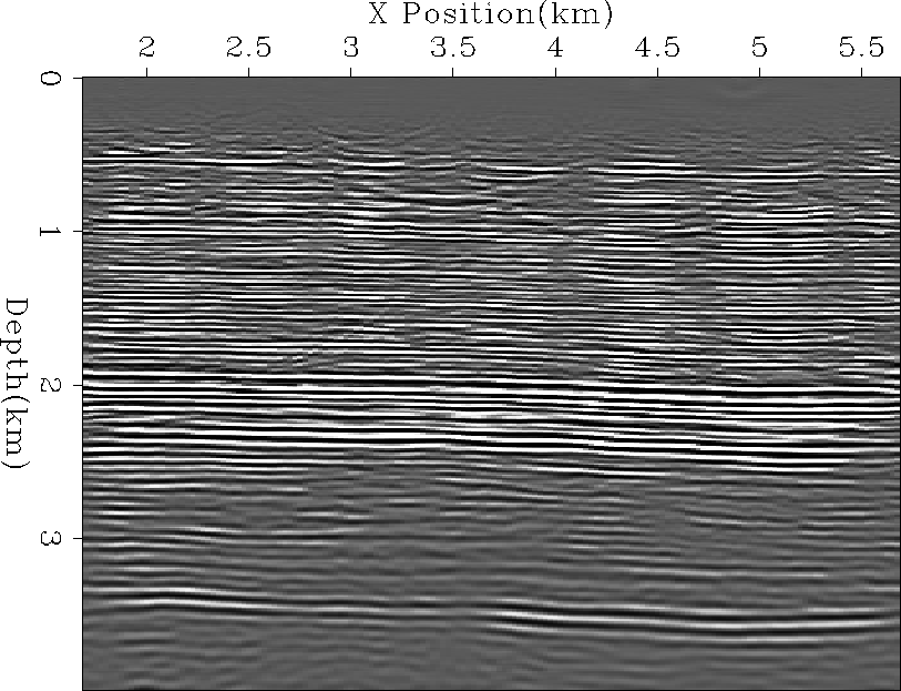
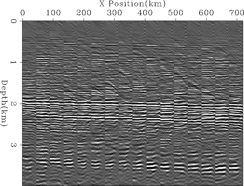
Figure 3 shows the resulting angle gathers Sava (2000).
Note how the image is generally well focused and the gathers with some
slight variation below three kilometers at x=3.5. Figure 4
shows the moveout of the gathers in Figure 3. Note
the traditional `W' pattern associated with the velocity anomaly
can be seen in cross-section at depth.
vel-init
Figure 1 Initial velocity model.
|
| 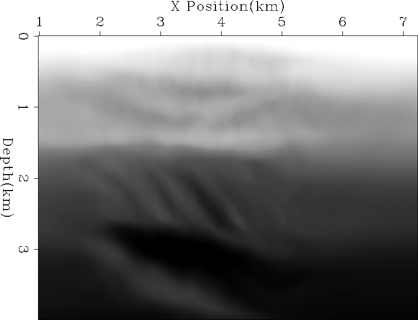 |


image-init
Figure 2 Initial migration using the velocity
shown in Figure 1.
|
|  |
mig-init
Figure 3 Every 10th migrated gather using the velocity
shown in Figure 1.
|
|  |
semb-init
Figure 4 Moveout of the gathers shown in Figure 3.
|
|  |
To start we need to solve the problem without accounting
for model variance.
If we solve for using fitting goals (4) our
updated velocity is shown in Figure 5. The change of
the velocity is generally minor, with an increase in the high
velocity structure at x=3.5, z=3.2. The resulting image
and migration gathers are shown in Figures 6
and 7. The resulting image is slightly
better focused below the anomaly and the migration gathers
are, as expected, a little flatter.
vel-none
Figure 5 New velocity obtained by inverting for
using fitting goals (4).
|
| 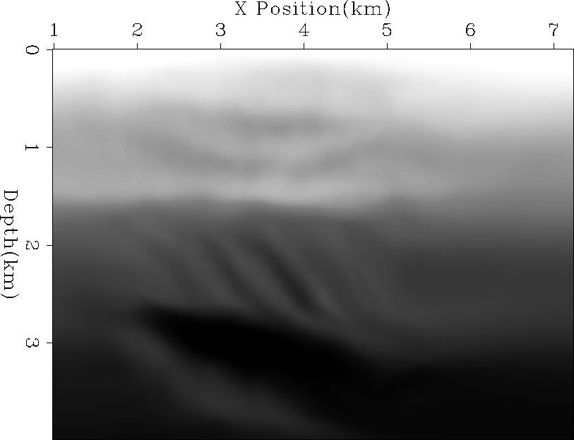 |
image-none
Figure 6 New image obtained by inverting for
using fitting goals (4) using the velocity shown in
Figure 5.
|
|  |
mig-none
Figure 7 New gathers obtained by inverting for
using fitting goals (4) using the velocity shown in
Figure 5.
|
|  |
If we apply equation (3) using the  when
estimating our improved velocity model we can find the
right amount of noise to add to our fitting goals. We can
now resolve for accounting for the model variability.
Figure 8 shows four such realizations.
Note that they have the same general structure as
seen in Figure 5 but within additional
texture that is accounted for by covariance description.
If we migrate with these new velocity models we get the
images and migrated gathers shown in Figures 9
and 10. In printed form these images appear
identical, or close to identical. If watched as a movie, amplitude
differences can be observed.
when
estimating our improved velocity model we can find the
right amount of noise to add to our fitting goals. We can
now resolve for accounting for the model variability.
Figure 8 shows four such realizations.
Note that they have the same general structure as
seen in Figure 5 but within additional
texture that is accounted for by covariance description.
If we migrate with these new velocity models we get the
images and migrated gathers shown in Figures 9
and 10. In printed form these images appear
identical, or close to identical. If watched as a movie, amplitude
differences can be observed.
vel-multi
Figure 8 Four different realizations of the velocity
accounting for model variability.
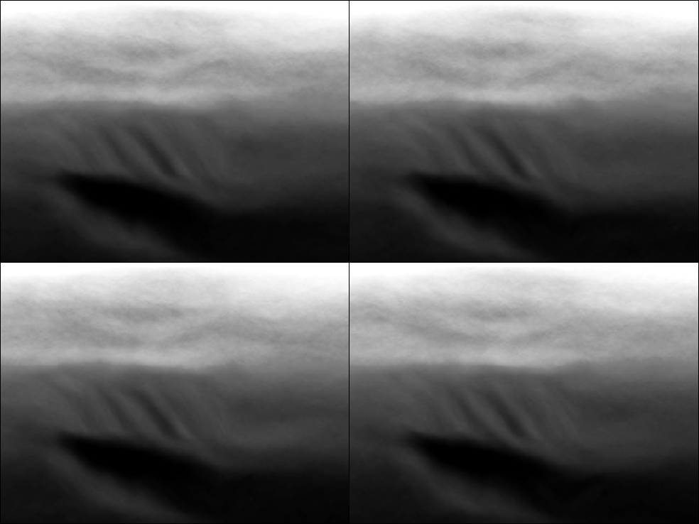
![[*]](http://sepwww.stanford.edu/latex2html/movie.gif) image-multi
image-multi
Figure 9 Four different realizations of the migration
accounting for model variability. Note how the reflector position is nearly
identical in each realization and with the image without variability (Figure 6), but the amplitudes vary slightly.
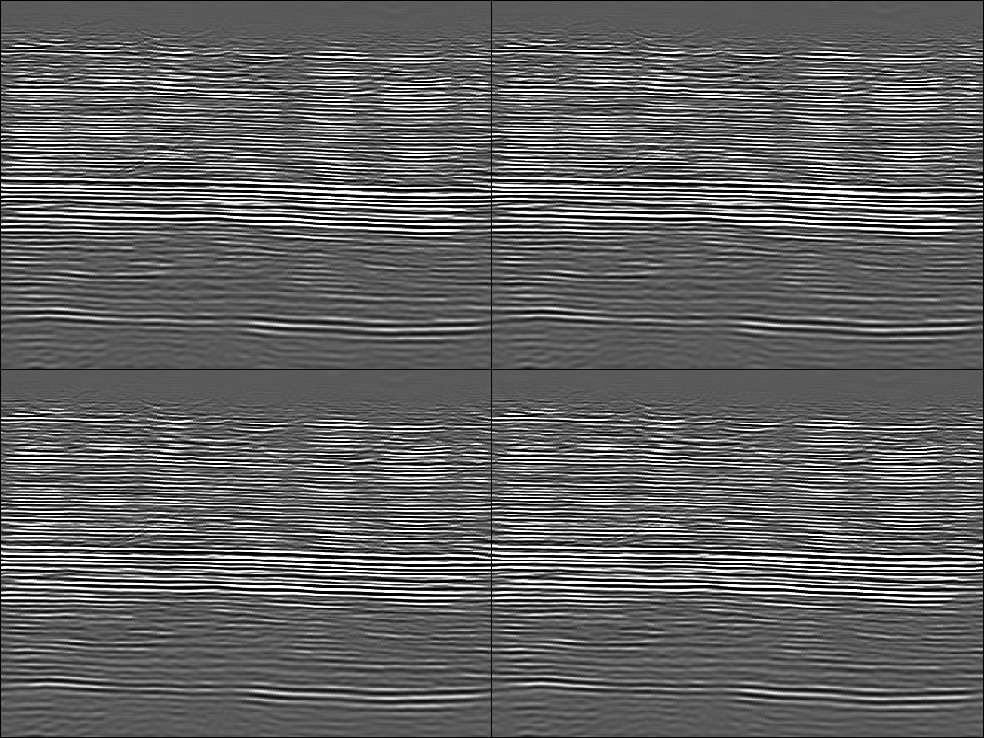
mig-multi
Figure 10 Four different realizations of the migration
accounting for model variability. Note how the reflector position is nearly
identical in each realization and with the image without variability (Figure 7).
Next: AVA analysis
Up: Clapp: Effect of velocity
Previous: Clapp: Effect of velocity
Stanford Exploration Project
6/8/2002