Implications to 4D

Accepting the previously outlined rock physics conundrum, we can now think about the implications of this creep behavior, and our ability to capture it in the lab, to the repeat seismic experiment. As most of the rock physics field has historically been dedicated to the application of acoustic manipulations and pressure dependencies there is much work available concerning the elastic sensitivities of rock, packs, and beads to various pressure regimes Mavko (2001). All of this understanding however hinges on the basic immutability of the mineral frame (elastic deformation) until a yield point from which a sample cannot recover (fracture or grain crushing).

 

pres Figure 9 Experiment illustrating the effective pressure law by increasing and decreasing effective pressure while keeping the pore pressure constant. Minor hysteresis observable, but obviously an elastic phenomenon.Mavko (2001)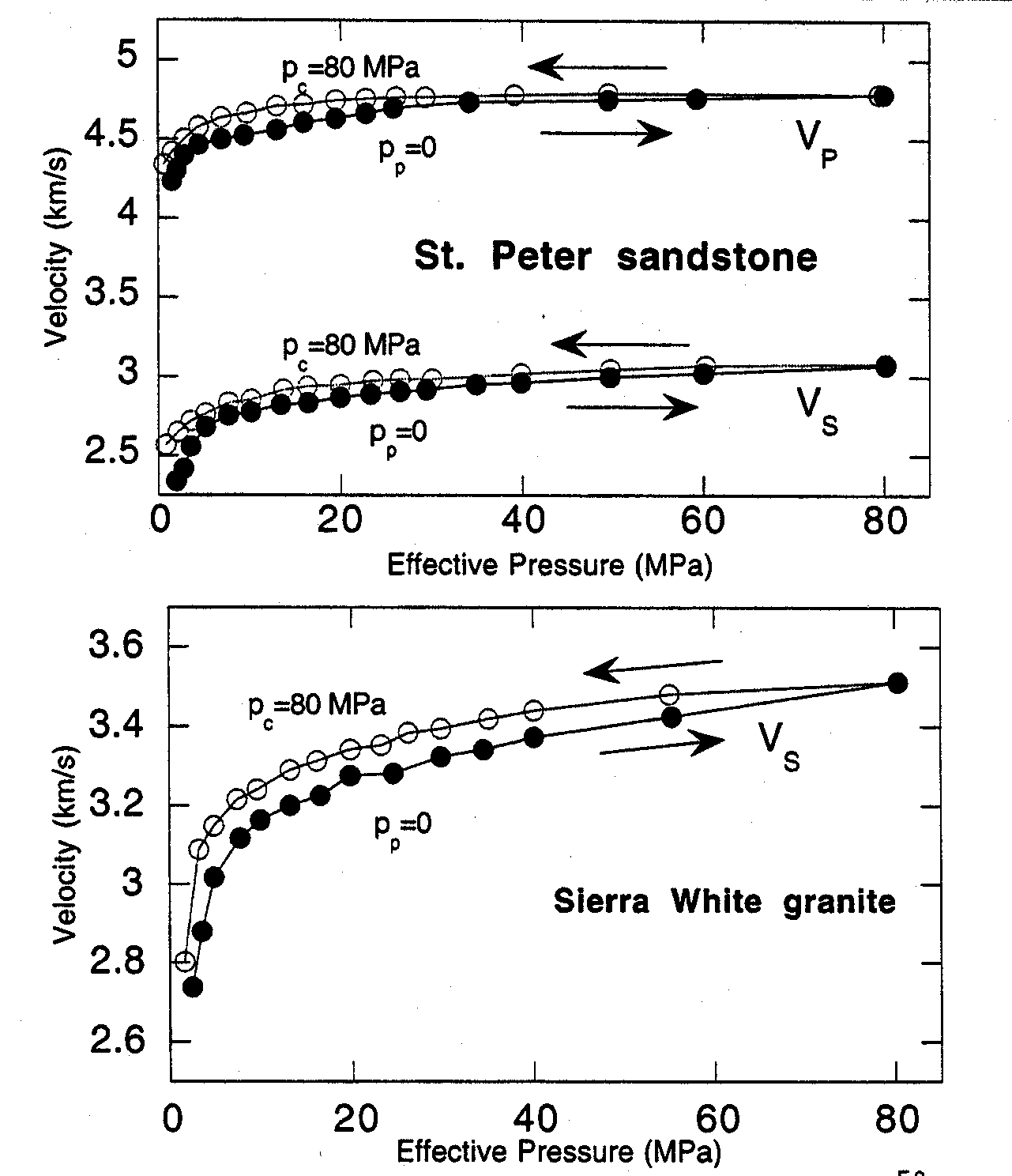

We begin to realize that our discussion thus far begins to impinge on the underlying assumption for the classic rock physics justifications for 4D seismic: namely that the rock frame does not change. The previous sections show that it does. Thus there are no constants to hold on to for any experiment, be they fluid substitution or seismic. We might as well be dealing with an entirely new reservoir.

 

sat Figure 10 Different micro-distributions of pore fluids and gas within the porosity of the rock frame significantly effect the velocity dependence on water saturation.Mavko (2001)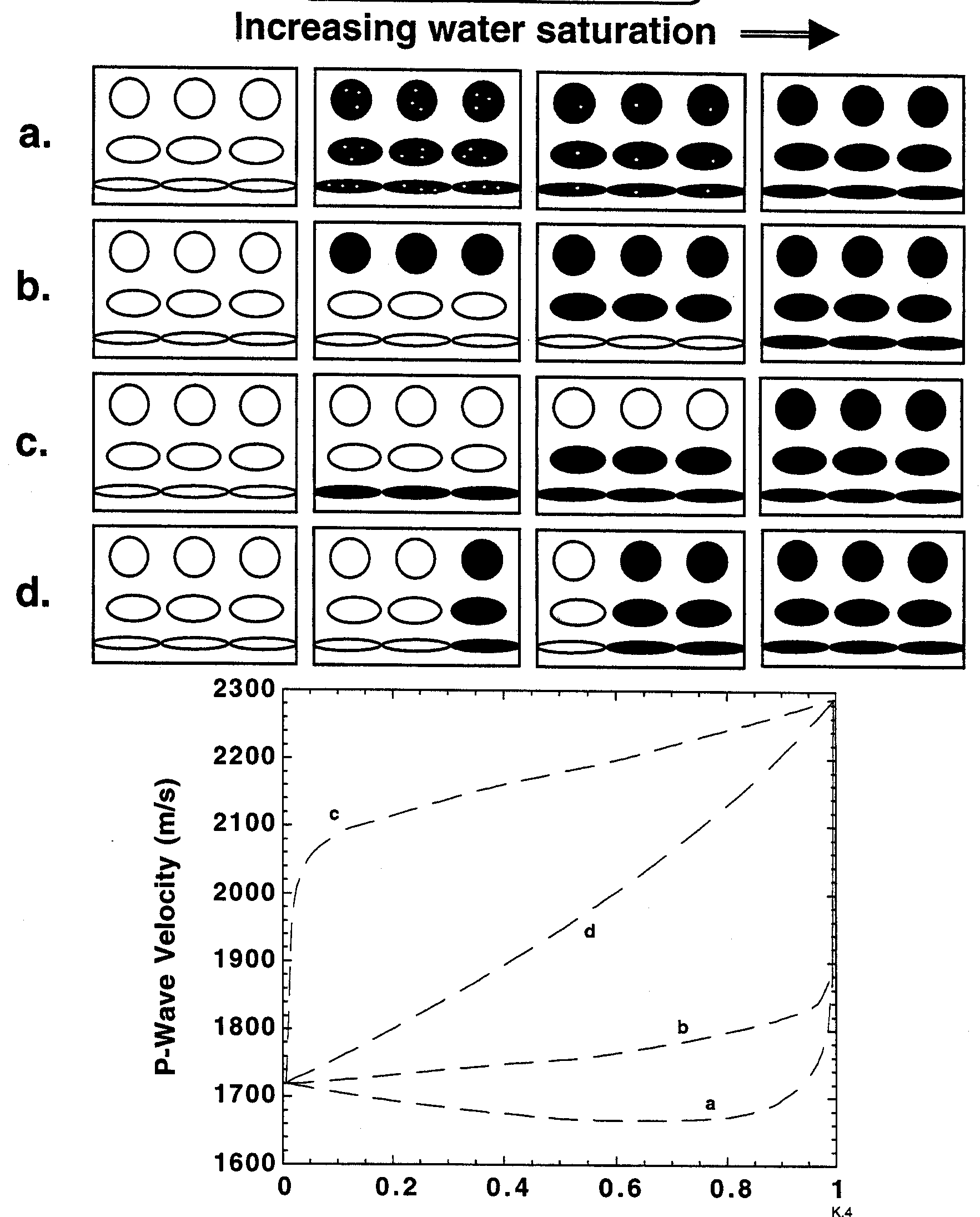

 

model Figure 11 If fluids and elastic pressure dependence are understood, the seismic evolution of a reservoir can easily be modeled with a few simple plots. Fluid substitution calculated in this instance with Gassman model from dry lab data.Mavko (2001)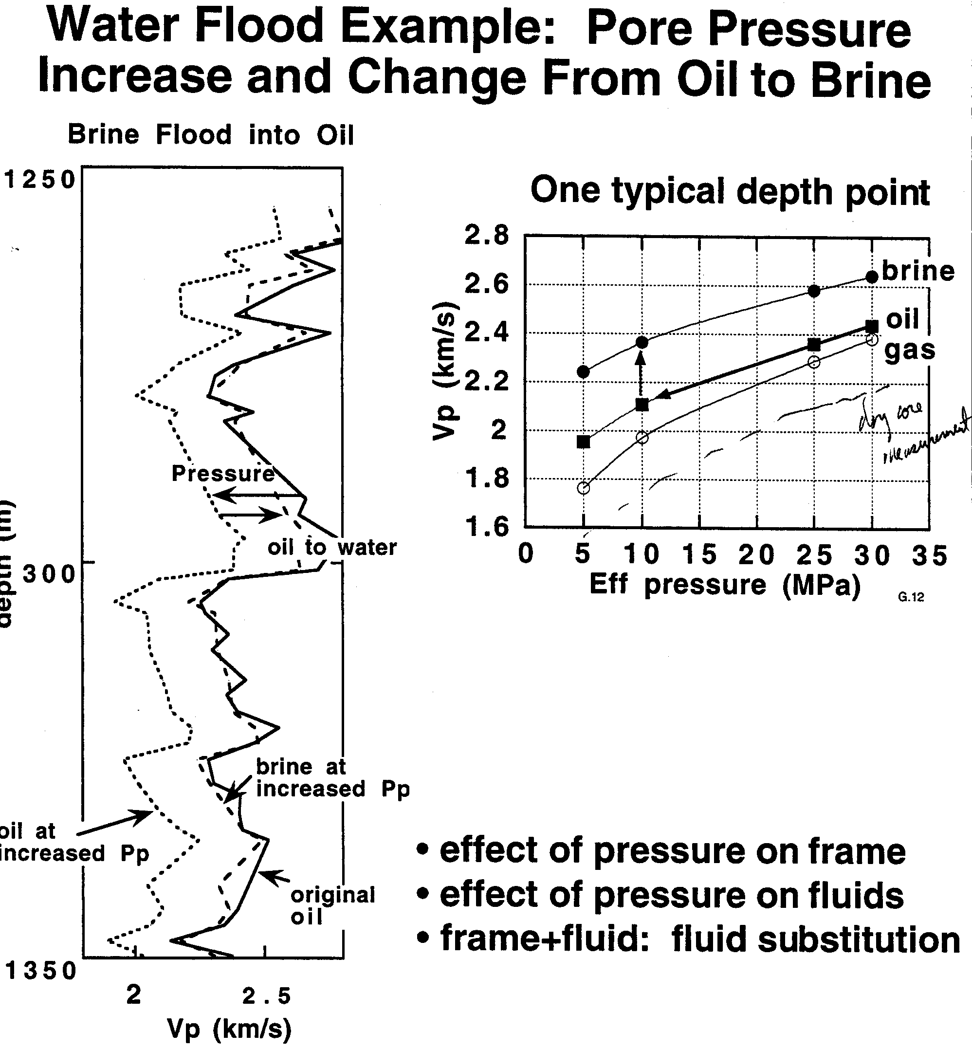

To add to the conclusions to the creep investigation section above, it is imperative to perform experiments to not only understand the creep mechanisms, but also their effects on sonic velocities or acoustic moduli. It is obvious that the various transformations depicted in Figure 8 will result in new elastic moduli as we are basically manufacturing a new rock sample.

This is quite troubling when the second conclusion of Juarez-Badillo creep behavior is remembered. Solving for $\epsilon_{final}/\tau$rather than for the two independently removes our ability to predict end-state compaction and the time (supposed to be analogous to production life of a reservoir) to achieve it. While this seemed a disappointing but not insurmountable obstacle previously, it could be a real show stopper in the 4D context.

To that end, the experiments mentioned previously need be undertaken with the addendum of velocity measurements along the way. It is very possible that while the samples can show time-scaling of creep mechanisms, parts of the distribution of mechanisms may indeed exhibit very different manifestations in elastic parameters.