


![[*]](http://sepwww.stanford.edu/latex2html/foot_motif.gif) that includes a very broad Gaussian range of parameters.
Juarez-Badillo (1985) showed a Cole-Cole type deformation model that will
be explored here to unite all of these observations.
that includes a very broad Gaussian range of parameters.
Juarez-Badillo (1985) showed a Cole-Cole type deformation model that will
be explored here to unite all of these observations.
The empirical relation developed by Juarez-Badillo is of the form
| |
(2) |
Knowing that we need to find a power-law form to fit the observations,
we can analyze this equation under the limit where the time of the
experiment, t, is much less than the characteristic compaction
time, ![]() , defined as when the sample has undergone exactly half of
the final strain limit. This seems appropriate as we are making
an effort to do lab experiments at much less than the time that we
imagine these processing happening in the field.
, defined as when the sample has undergone exactly half of
the final strain limit. This seems appropriate as we are making
an effort to do lab experiments at much less than the time that we
imagine these processing happening in the field.
Equation 2 then becomes
![]()
![]()
We notice now that the strain at time 1
![]()
and therefore
| |
(3) |
Not only does this equation fit well with the observed data, but
considering only progressive quartiles of the data, constant and stable
values for the regressed parameters ![]() and d are
obtained. This provides further justification in the selection of this
model as this was one of the significant problems with use of the
other models.
and d are
obtained. This provides further justification in the selection of this
model as this was one of the significant problems with use of the
other models.
Now, assuming that our adoption of the Juarez-Badillo creep mechanism is correct, we have a model that helps explain our data. This fit implies several things:
|
year
Figure 4 One year hold uniaxial creep test. Exponential function still fits meaning | 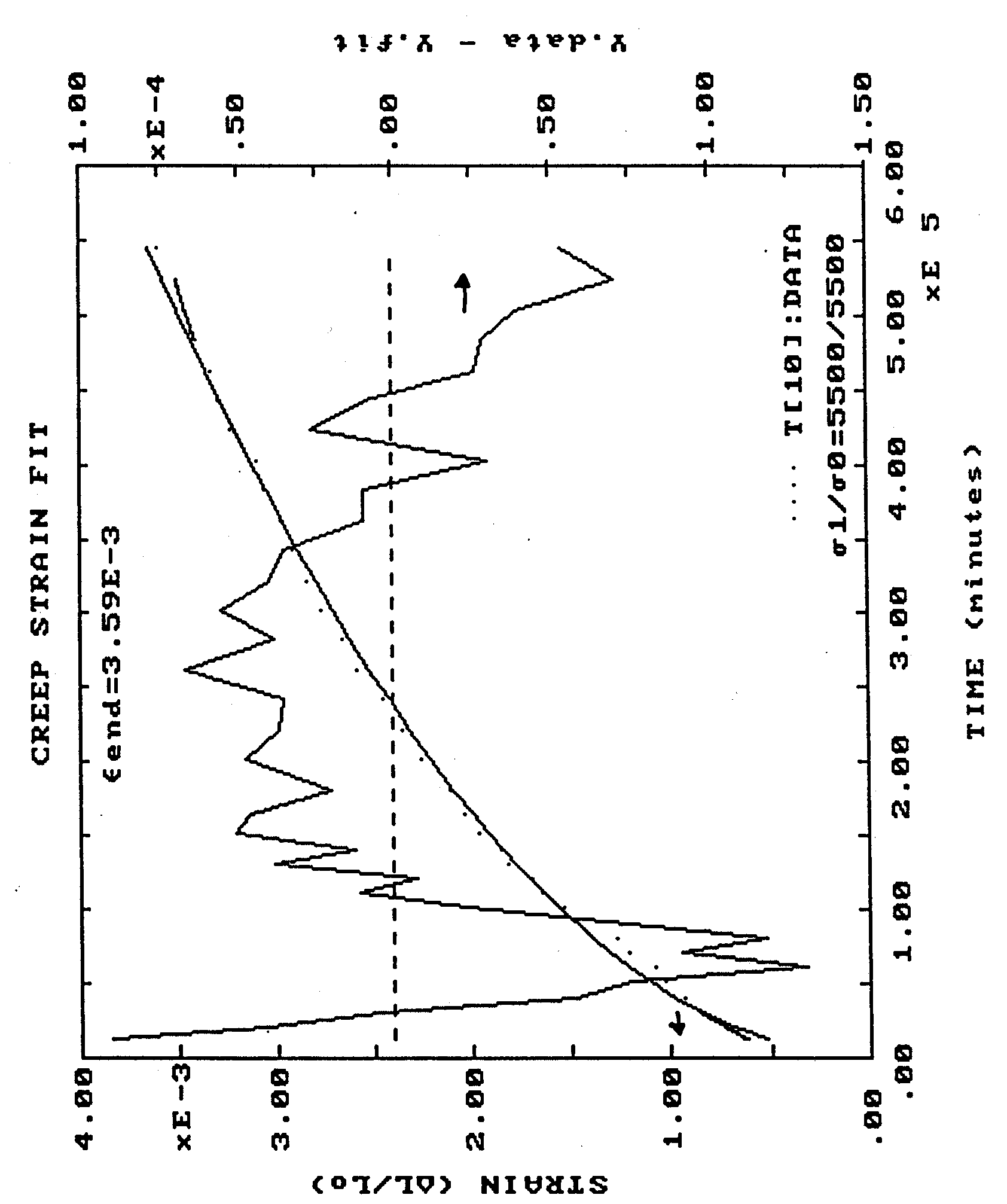 |
