Model space weighting methods

Another approach of approximating the inverse and the a posteriori covariance matrix is provided by the work of Claerbout and Nichols (1994). Rather than trying to solve the explicit inverse problem the adjoint of $\mathbf{A}$ is applied to the data, and a diagonal operator $\mathbf{W^2_m}$ is constructed, such that  

$$\Delta \mathbf{m}= \mathbf{W^2_m} \mathbf{A}^{T} \Delta \mathbf{d},$$ (6)

in which $\mathbf{W^2_m}$ is related to the model space weighting. This term is needed to obtain the correct physical units. Note that this term also corresponds to the a posteriori covariance. The most significant properties of the model space weighting term can be explored by measuring its effects when applied to a reference model $\Delta \mathbf{m_{ref}}$.For example, if $\mathbf{W^2_m}$ is given by  

$$\mathbf{W^2_m} =\frac {\mathbf{diag}\left(\Delta \mathbf{m_{... ...}\right)} \approx \left(\mathbf{A}^{T}\mathbf{A} \right)^{-1},$$ (7)

will have the same units as $\mathbf{A}^{\dagger}$, and the properties of this term can be explored. Two choices of $\Delta \mathbf{m_{ref}}$ will be shown here (Biondi, 1998):

• $\Delta \mathbf{m_{ref}}=$unity vector
• $\Delta \mathbf{m_{ref}}=$unit vector e^k in k direction in m-D (k=1,2,...,m)

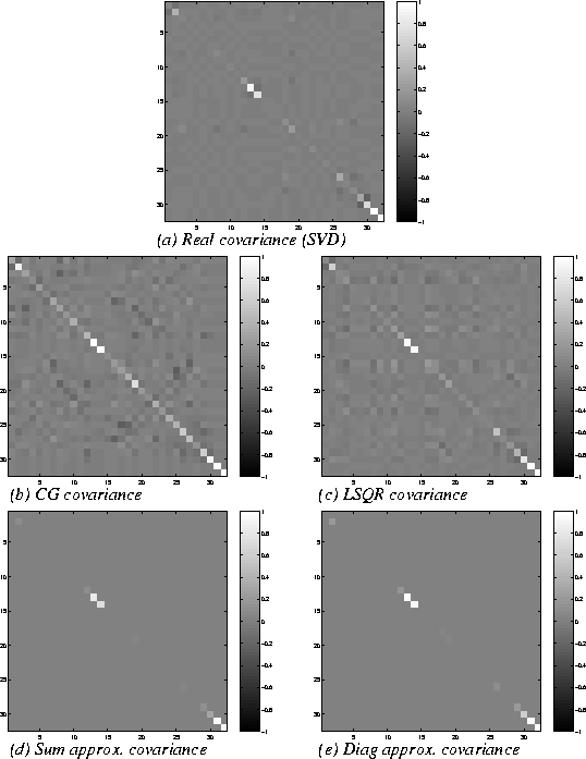
The first choice results in the sum of the elements in each column of $\mathbf{A}$ in the denominator. The second choice results in the sum of the square of the elements in each column of $\mathbf{A}$ in the denominator. The obtained vector forms the diagonal in the approximated $\left( \mathbf{A}^T \mathbf{A} \right)^{-1}$. Figure 9d,e shows a posteriori covariance matrices for M=33 model parameters obtained by respectively the "sum" approximation and the "diagonal" approximation. Note that only the diagonal elements are calculated. These elements resemble the diagonal of the real a posteriori covariance matrix (Fig.9a).

Whether the iterative methods, or the model space weighting methods should be used for calculation of the covariance matrix depends also on the algorithm that is used for calculating the approximate inverse. In general, iterative methods are used for tomography, and the vectors needed for calculation of the covariance are obtained without any extra costs. The calculated covariance matrix will reflect the status of the inversion after the performed number of iterations. However, a drawback of these methods is that the solution space vectors need to be saved after each iteration. Moreover, not performing enough iterations might result in strange covariance matrix. Nevertheless, this matrix will still reflect the status of your inversion after the performed number of iterations. The model weight methods are very cheap, and give accurate results of the diagonal elements of the covariance. Nevertheless, the non-diagonal elements are not calculated. However, as for the re-parameterization only this diagonal is considered, these methods might be sufficient. When the covariance between the different parameters is going to play a role in the inversion too, the full covariance matrix obtained from the iterative methods should be used.

 

covariance
Figure 9 (a) Real covariance matrix calculated by SVD; (b)(c) Covariance matrices approximated by iterative methods; (d)(e) Covariance matrices approximated by model space weight methods.