Shot-profile migration and modeling

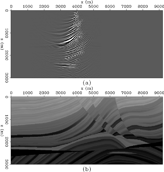
Shot-profile migration is similar to exploding-reflector migration, except individual shot records are migrated independently. Single shot-record migrations (like Figure ) are then stacked to provide a complete reflectivity image.

 

singleshot Figure 1 A single migrated shot record (a) over the Marmousi Bourgeois et al. (1991) velocity model (b).

Rather than downward-continue a single wavefield into the earth, we downward-continue two wavefields simultaneously (but still one frequency at a time). Firstly, there is upgoing wavefield (${\bf q}_{\omega,s}^{+}$), which was recorded on the surface as the shot-gather, ${\bf d}_{\omega,s}$,with a shot at s. The equation for downward continuing this wavefield is:  

$${\bf D}_{\omega} \; {\bf q}_{\omega,s}^{+} = {\bf Z} \; {\bf d}_{\omega,s},$$ (71)

Secondly, there is the downgoing wavefield (${\bf q}_{\omega,s}^{-}$),  

$${\bf D}_{\omega} \; {\bf q}_{\omega,s}^{-} = {\bf Z} \; {\bf \delta}_{\omega,s},$$ (72)

which we did not record on the surface but we can simulate as an impulse at the shot location, ${\bf \delta}_{\omega,s}$.

To image an individual shot, we crosscorrelate the two wavefields and extract the image at zero-time, or equivalently multiply their Fourier coefficients and sum over frequencies. The matrix operation described by this process is,

$$\left( \matrix{ \hat{\bf m}_{1,s} \cr \hat{\bf m}_{2,s} \cr ... ...}^{+} \cr ...\cr {\bf q}_{\omega_{N_\omega}^{+}} \cr } \right).$$ (73)

To image the entire survey we then stack over shot-location. Full prestack shot-profile migration is therefore described by the equation  

$$\hat{\bf m} = {\bf \Sigma}_{s} \; {\bf \Sigma}_{\omega} \;... ... {\bf Z}_{N_\omega N_s} {\bf d} = {\bf A}'_{\rm SP} \; {\bf d}.$$ (74)

where ${\bf Q}_{-}$ = ${\bf diag}({\bf q}^{-})$, and ${\bf A}'_{\rm SP}$is the composite shot-profile migration operator.

The adjoint of equation () describes a process of common-shot modeling:  

$$\hat{\bf d} = {\bf Z}'_{N_\omega N_s} \; ({\bf D}')^{-1} \;... ...; {\bf \Sigma}_{s}' \; {\bf m} = {\bf A}_{\rm SP} \; {\bf m}.$$ (75)

Implementing equation () is slightly more difficult than equation (), since we cannot downward continue both wavefields from the surface simultaneously. However, we can still work with frequency slices; although for each frequency we must downward continue the shot wavefield from the surface to the bottom of the model storing it as we go, and then upward continue the reflected wavefield to the surface.