Amplitude correction in constant velocity

Migration is, by the standard definition, the operation adjoint to forward modeling. It is performed by the downward continuing the recorded wavefield and imaging at zero time:  

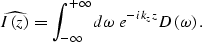$$\widehat{ I\left (z \right )}= \int_{-\infty}^{+\infty} d\omega \; e^{-ik_zz} D\left (\omega\right ).$$ (3)

We substitute Equation (1) into Equation (3), and expand the integral in Equation (1) to negative depth, for which the image is zero, by definition:

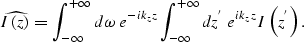$$\widehat{I\left (z \right )} = \int_{-\infty}^{+\infty} d\om... ...-\infty}^{+\infty} dz^{'} \; e^{ ik_zz} I\left (z^{'} \right ).$$ (4)

We then change the integration variable $\omega$ to k_z and obtain:  

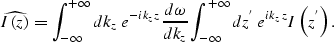$$\widehat{I\left (z \right )} = \int_{-\infty}^{+\infty} dk_z... ...-\infty}^{+\infty} dz^{'} \; e^{ ik_zz} I\left (z^{'} \right ).$$ (5)

The pair of integrals in Equation (5) describe forward and inverse Fourier transforms, and thus the effect of chaining modeling and migration on the image is simply the equivalent of applying the Jacobian $d\omega/dk_z$.This result is valid only for real values of k_z, which is what we want, since we are not interested in the wavefield component for which k_z becomes imaginary (that is, we neglect evanescent waves).

In constant velocity, the frequency-wavenumber representation of the Jacobian is simply a multiplication:

$$\begin{eqnarray} \widehat{ I\left (k_z\right )} &=& \frac{d\omega}{dk_z} I\left ... ... &=& \frac{d\omega}{dk_z} G\left (k_z\right )R\left (k_z\right ).\end{eqnarray}$$ (6)

The Jacobian weighting is introduced by the imaging step, therefore, the Jacobian depends on the coordinates used to define the wavefield during imaging: constant ray-parameter or constant offset wavenumber.

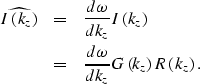
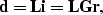
In matrix notation, Equation (1) is written  

$$\bold d= \bold L\bold i= \bold L\bold G\bold r,$$ (7)

where $\bold d$, $\bold i$, and $\bold r$ are respectively the data, image, and reflectivity vectors, $\bold G$ is a diagonal matrix representing the reflection operator, and $\bold L$ is the modeling operator. With this notation, Equation (5) becomes  

$$\widehat{\bold i}= \bold L^{*} \bold d= \bold L^{*}\bold L\bold i= \bold W\bold i= \bold W\bold G\bold r,$$ (8)

where $\bold W$ is a diagonal matrix representing the Jacobian $d\omega/dk_z$.