Jacobian for Common-azimuth migration

The dispersion relation of 3-D common-azimuth migration can be written as a cascade of 2-D inline prestack migration and 2-D zero-offset crossline migration Biondi (1999):

$$\begin{eqnarray} k_{z_{x}}&=& {\rm SSR}{{k_m}_x-{k_h}_x} + {\rm SSR}{{k_m}_x+{k_h}_x} \nonumber \\ k_z^{\rm CA}&=& \sqrt{k_{z_{x}}^2 - k_{y_m}^2}.\end{eqnarray}$$ (32)

We can derive the expression for the common-azimuth Jacobian by simply applying the chain rule to Equation (32):

$$\frac{dk_z^{\rm CA}}{d\omega} = \frac{dk_z^{\rm CA}}{dk_{z_{x}}} \frac{dk_{z_{x}}}{d\omega}.$$ (33)

If we note that

$$\frac{dk_z^{\rm CA}}{dk_{z_{x}}} = \frac{k_{z_{x}}}{k_z^{\rm CA}}$$ (34)

we obtain the common-azimuth Jacobian:

$$\bold W^{\rm CA}= \frac{k_z^{\rm CA}}{k_{z_{x}}} \bold W^{\rm 2D}$$ (35)

where $\bold W^{\rm 2D}$ is the 2-D version of the Jacobian we derived in the preceding sections, either for reflection-angle ADCIGs, Equation (23), or for offset ray-parameter, Equation (28).

However, computing the reflection operator weight, Equation (2), and the WKBJ amplitudes, Equation (11), requires us to evaluate separately the source ${k_{\rm zs}}$ and receiver ${k_{\rm zr}}$ components of the dispersion relation. Therefore, for the ``true-amplitude'' migration weights, Equation (12), we need to use the more complicated expression for the common-azimuth dispersion relation as introduced by Biondi and Palacharla (1996).

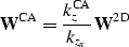
In addition to the amplitude terms we have discussed in the preceding sections, ``true-amplitude'' common-azimuth migration requires an additional correction that takes into account that its dispersion relation is obtained by a stationary-phase approximation of the full 3-D DSR equation. We, therefore, need to augment the amplitude term in Equation (9) by another factor, which results from stationary-phase approximation theory Bleistein and Handelsman (1975):  

$$\AA_{\rm{stat}} = \sqrt{\frac{2\pi}{\int\limits_{0}^{z}\left... ...left (\frac{d^2k_z^{\rm CA}}{dk_{y_h}^2}\right )\frac{\pi}{4}},$$ (36)

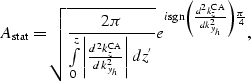
where the second derivative of $k_z^{\rm CA}$ with respect to k_yh is:

$$\begin{eqnarray} \frac{d^2k_z^{\rm CA}}{dk_{y_h}^2} = &-&\frac{ \left (2\omega ... ...t )^2 - \left ({k_m}_y+\widehat{{k_h}_y}\right )^2 \right ]^{3/2}}\end{eqnarray}$$ (37)

with  

$$\widehat{k_{y_h}}= k_{y_m}\frac {{\rm SSR}{{k_m}_x+{k_h}_x} ... ...} } {{\rm SSR}{{k_m}_x+{k_h}_x} + {\rm SSR}{{k_m}_x-{k_h}_x} }.$$ (38)

This additional correction factor includes both a phase shift component and an amplitude component which increases with depth. It has thus a behavior similar to the correction term that is often used to transform 2-D data recorded with point sources and receivers to 2-D data recorded with line sources and receivers Clayton and Stolt (1981). The physical explanation is also analogous: Common-azimuth migration assumes that the data were recorded for all values of the crossline offset (y_h) and then stacked along y_h. The inverse of $\AA_{\rm{stat}}$transforms the data recorded at zero crossline offset into the data ``expected'' by common-azimuth migration.

Figures 14-16 demonstrate the effects of applying the different weights in common-azimuth migration. These images are obtained by migrating a synthetic data set containing five dipping reflectors with dips from 0 to 60 degrees Biondi (2001).

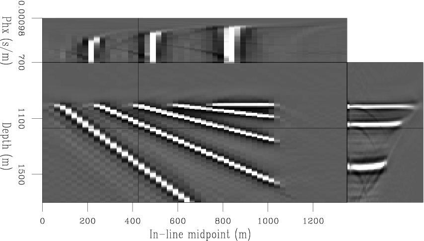
Figure 14 shows a subset of the migration results. The front face of the cube displayed in the figure is an in-line section stacked over p_h. The other two faces are sections through the prestack image as a function of the offset ray parameter (p_h). Those images are obtained by migration without any weighting factors. Figure 15 shows the same subset as in Figure 14, but obtained by applying all the appropriate weights and the phase shift related to the stationary-phase approximation. The weights balance the amplitudes along the reflector, so that the dipping reflectors are comparable with the flat one.

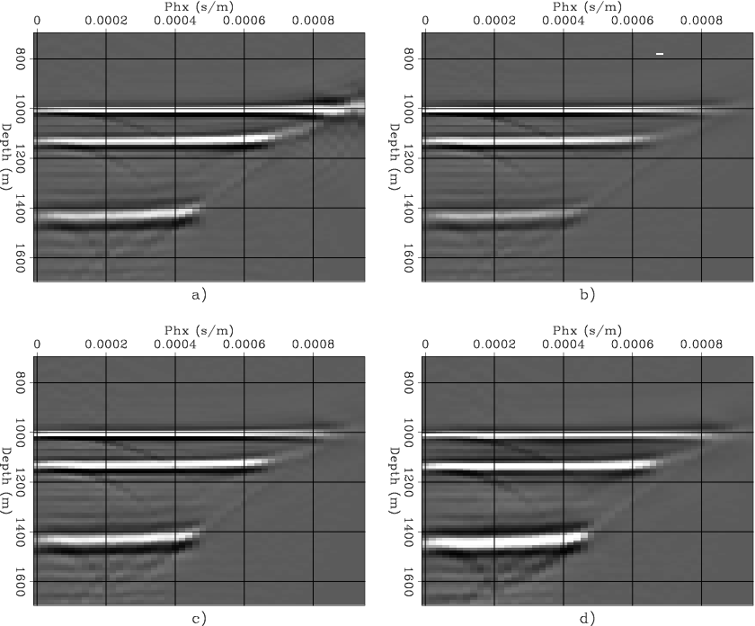
Figure 16 shows one particular ADCIG, detailing the effects of each type of weighting: no weights (Figure 16a), Jacobian and modeling weights (Figure 16b), Jacobian, modeling and WKBJ weights (Figure 16c), and Jacobian, modeling, WKBJ and phase-shift weights (Figure 16d).

 

CA-pull-none-vp
Figure 14 A subset of the results of common-azimuth migration of the synthetic data set. The front face of the cube is an in-line section stacked along p_h. The other two faces are sections through the prestack image. The migrated cube is obtained from migration without any weighting. The amplitudes of the dipping reflectors are lower than expected, and the whole image has the wrong phase.

 

CA-pull-WKBJ-stat-vp
Figure 15 A subset of the results of common-azimuth migration of the synthetic data set. The front face of the cube is an in-line section stacked along p_h. The migrated cube is obtained from migration with all the appropriate weights and the stationary-phase phase shift. The amplitudes of the dipping reflectors are comparable with those of the flat reflector, and the whole image has the correct phase.

 

CIG-amp
Figure 16 ADCIGs obtained by common-azimuth migration with different amplitude weights: a) No weights, b) $G^{-1} {\bold W_{p_{x_h}}^{\rm CA}}^{-1}$ (Jacobian), c) $G^{-1}\AA^{-1}{\bold W_{p_{x_h}}^{\rm CA}}^{-1}$ (Jacobian and WKBJ), d) $\AA_{\rm stat}^{-1}G^{-1}\AA^{-1}{\bold W_{p_{x_h}}^{\rm CA}}^{-1}$ (Jacobian, WKBJ, and stationary phase). The relative amplitudes of the dipping reflectors are modified by the different migration weights.