Least Squares Formulation

The fundamental data unit of this paper is the ``time/depth pair'', which is quite simply the traveltime of seismic waves to a specified depth, along an assumed vertical raypath. We denote time depth pairs by ($\tau_p, \zeta_p$), indexed by p, the ``pair'' index. The output velocity function is linear within layers. We denote layer boundaries, which are independent of the time/depth pairs, by t_l, indexed by l, the ``layer'' index.

We begin by deriving the 1-D data residual - the depth error between the depth component of a time/depth pair ($\zeta_p$) and its time component ($\tau_p$) after vertical stretch with the (unknown) interval velocity:  

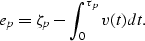$$e_p = \zeta_p - \int_{0}^{\tau_p} v(t) dt.$$ (1)

For implementation purposes, we break the integral into the sum of integrals between neighboring time/depth pairs ($t=[\tau_p,\tau_{p+1}]$):  

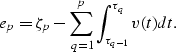$$e_p = \zeta_p - \sum_{q=1}^p \int_{\tau_{q-1}}^{\tau_q} v(t) dt.$$ (2)

We assume that the interval velocity in layer l is linear,

$$v(t) = v_{0,l} + k_l t; \hspace{0.25in} \left\{ t=[t_l,t_{l+1}] \right\},$$ (3)

so the integral in equation (2) has a closed form. To obtain a correspondence between time/depth pairs and layer boundaries, note that, given a time/depth pair, we can always determine in which layer it resides. In other words, we can unambiguously write l as a function of p, l[p]. Now we can evaluate the integrals of equation (2):  

$$e_p = \zeta_p - \sum_{q=1}^{p} v_{0,l[q]}(\tau_{q+1}-\tau_q) + \frac{k_{l[q]}}{2}(\tau^2_{q+1}-\tau^2_q).$$ (4)

Equation (4) defines the misfit for a single time/depth pair, as a function of the model parameters. Now pack the individual misfits from equation (4) into a residual vector, $\bold r_d$:  

$$\bold r_d = {\boldsymbol \zeta} - \bold A \left[\begin{array} {c} \bold v_0 \\ \bold k \end{array}\right] \approx \bf 0$$ (5)

The elements of vector $\boldsymbol \zeta$ are the time/depth pair depth values, $\bf A$ is the summation operator suggested by equation (4). and $[\bold v_0 \;\; \bold k]^T$ is the unknown vector of intercept and slope parameters. The primary goal of least squares optimization is to minimize the mean squared error of the data residual, hence the familiar fitting goal ($\approx$) notation.