


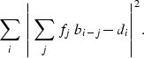
 |
(1) |
With the notation that ![]() is the matrix representing
convolution with time series
is the matrix representing
convolution with time series ![]() , we can rewrite this desired
minimization as a fitting goal [e.g. Claerbout (1998a)],
, we can rewrite this desired
minimization as a fitting goal [e.g. Claerbout (1998a)],
| (2) |
| |
(3) |
For the multiple suppression problem, the vector ![]() represents
the multiple infested raw data, and the matrix
represents
the multiple infested raw data, and the matrix ![]() represents
convolution with the multiple model.
Criterion (1) implies a choice of filter
represents
convolution with the multiple model.
Criterion (1) implies a choice of filter
![]() that minimizes the energy in the dataset after multiple
removal.
that minimizes the energy in the dataset after multiple
removal.
One advantage with working with time-domain filters as opposed to
frequency-domain filters is that the theory can be adapted relatively
easily to address non-stationarity.
Following Claerbout (1998a) and Margrave (1998), we extend the
concept of a filter to that of a non-stationary filter-bank, which in
principle contains one filter for every point in the input/output
space.
For a non-stationary filter-bank, ![]() , we identify
, we identify ![]() with the filter corresponding to the
with the filter corresponding to the ![]() location in the
input/output vector, and the coefficient, fi,j, with the
location in the
input/output vector, and the coefficient, fi,j, with the
![]() coefficient of the filter,
coefficient of the filter, ![]() .The response of non-stationary filtering with
.The response of non-stationary filtering with ![]() to an impulse
in the
to an impulse
in the ![]() location in the input is then
location in the input is then ![]() .
.
With a non-stationary convolution filter, ![]() , the shaping
filter regression normal equations,
are massively underdetermined since there is a potentially unique
impulse response associated with every point in the dataspace.
We need additional constraints to reduce the null space of the
problem.
, the shaping
filter regression normal equations,
are massively underdetermined since there is a potentially unique
impulse response associated with every point in the dataspace.
We need additional constraints to reduce the null space of the
problem.
For most problems, we do not want the filter impulse responses to vary arbitrarily, we would rather only consider filters whose impulse response varies smoothly across the output space. This preconception can be expressed mathematically by saying that, simultaneously with expression (1), we would also like to minimize
 |
(4) |
Combining expressions (1) and (4)
with a parameter, ![]() that describes their relative importance,
we can write a pair of fitting goals
that describes their relative importance,
we can write a pair of fitting goals
| |
(5) | |
| (6) |
By making the change of variables,
![]() Fomel (1997),
we obtain the following fitting goals
Fomel (1997),
we obtain the following fitting goals
| |
(7) | |
| (8) |
| |
(9) |