Antialiasing conditions for the PRT operator

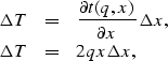
Antialiasing the operator is equivalent to dip-filtering the operator. The anti-aliasing conditions can be written Abma et al. (1999) as

$$f_{max} \leq \frac{1}{2\Delta T},$$ (9)

where $\Delta T$ is the local slope of the operator between two adjacent traces. For the PRT, we can compute the local slope as follows:

$$\begin{eqnarray} \Delta T &=& \frac{\partial t(q,x)}{\partial x} \Delta x, \\ \Delta T &=& 2qx \Delta x,\end{eqnarray}$$ (10) (11)

where $\Delta x$ is the input trace spacing. The antialiasing condition becomes

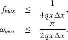$$\begin{eqnarray} f_{max} &\leq& \frac{1}{4qx\Delta x}, \\ \omega_{max} &\leq& \frac{\pi}{2qx \Delta x}.\end{eqnarray}$$ (12) (13)

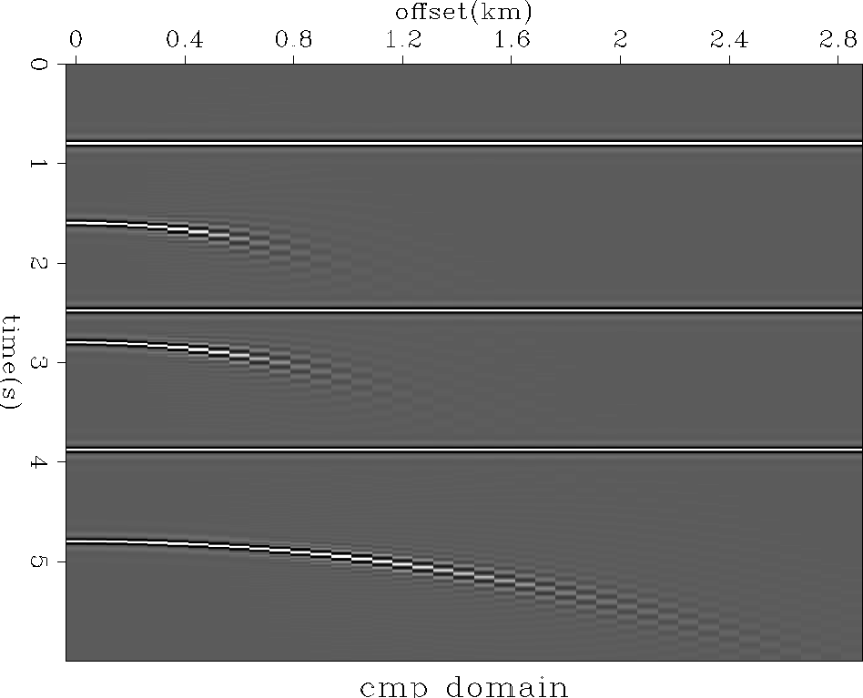
The antialiasing condition in equation (13) is then implemented in the Fourier domain. Figure 3 shows how the antialiasing works in the data space when the adjoint of the PRT (${\bf L'}$) is applied to the model in Figure 1: parabolas broaden with offset as a result of the dip filtering. Thus, the antialiasing operator generates a loss of resolution.

 

data_spikena Figure 3 Effects of antialiasing in the data space. The parabolas broaden with offset as a result of the low-pass filtering for large qs.

We now apply the antialiasing operator to the CMP gather shown in the right-hand panel of Figure 1. The radon domain in Figure 4 (as compared with that in Figure 2) has been cleaned up with a loss of resolution. However, because we apply an antialiasing operator with aliased data, we are left with aliasing noise near q=0 s/km². This aliasing noise is caused by the aliasing of the non-flat events in the CMP domain. We can mitigate these artifacts by introducing some constraints in the radon domain as a function of the expected aliased dips in the data Biondi (1998), but this is not considered here. Nonetheless, we see that the use of an antialiasing operator with aliased data is worthwhile. In addition, cleaning up the aliasing artifacts for a high q is particularly interesting when multiples are present in the data. Indeed, multiples, often aliased in the CMP domain, map in regions of high q where the antialiasing operator is the most efficient.

In the next section, I investigate the effects of the antialiasing operator when the radon domain is derived with a least-squares approach.

 

noal
Figure 4 Left: The parabolic radon domain after use of the antialising condition. The aliasing artifacts have decreased. Right: The reconstructed data after the forward operator is applied to the left panel.