

Next: 3-D missing data interpolation
Up: Plane-wave destruction in 3-D
Previous: Plane-wave destruction in 3-D
Let us denote the coordinates of a three-dimensional space by t,
x, and y. A theoretical plane wave is described by the equation
|  |
(116) |
where f is an arbitrary function, and  and
and  are
the plane slopes in the corresponding direction. It is easy to verify
that a plane wave of the form (
are
the plane slopes in the corresponding direction. It is easy to verify
that a plane wave of the form (![[*]](http://sepwww.stanford.edu/latex2html/cross_ref_motif.gif) ) satisfies the following
system of partial differential equations:
) satisfies the following
system of partial differential equations:
|  |
(117) |
The first equation in (![[*]](http://sepwww.stanford.edu/latex2html/cross_ref_motif.gif) ) describes plane waves on the
) describes plane waves on the
 slices and is completely equivalent to
equation (
slices and is completely equivalent to
equation (![[*]](http://sepwww.stanford.edu/latex2html/cross_ref_motif.gif) ). In its discrete form, it is represented as
a convolution with the two-dimensional finite-difference filter
). In its discrete form, it is represented as
a convolution with the two-dimensional finite-difference filter
 from equation (
![[*]](http://sepwww.stanford.edu/latex2html/cross_ref_motif.gif) ). Similarly, the second
equation transforms into a convolution with filter
). Similarly, the second
equation transforms into a convolution with filter  , which
acts on the
  slices. The discrete (finite-difference) form of
equations (
slices. The discrete (finite-difference) form of
equations (![[*]](http://sepwww.stanford.edu/latex2html/cross_ref_motif.gif) ) involves a blocked convolution operator:
) involves a blocked convolution operator:
| ![\begin{displaymath}
\left[\begin{array}
{c}\displaystyle
\bold{C}_x \\ \bold{C}_y\end{array}\right]\,\bold{m} = \bold{0}\;,\end{displaymath}](img232.gif) |
(118) |
where  is the model vector corresponding to P(t,x,y).
As follows from the theoretical analysis of the data regularization
problem in Chapter ![[*]](http://sepwww.stanford.edu/latex2html/cross_ref_motif.gif) , regularization implicitly
deals with the spectrum of the regularization filter, which
approximates the inverse model covariance. In other words, it involves
the square operator
, regularization implicitly
deals with the spectrum of the regularization filter, which
approximates the inverse model covariance. In other words, it involves
the square operator
| ![\begin{displaymath}
\left[\begin{array}
{cc}\displaystyle \bold{C}_x^T & \bold{C...
...\right] =
\bold{C}_x^T \bold{C}_x + \bold{C}_y^T \bold{C}_y\;.\end{displaymath}](img233.gif) |
(119) |
If we were able to transform this operator to the form
 , where
  is a three-dimensional
minimum-phase convolution, we could use the three-dimensional filter
 in place of the inconvenient pair
  and
and
 .
.
The problem of finding  from its spectrum is the familiar
spectral factorization problem. In fact, we already encountered a
problem analogous to (
from its spectrum is the familiar
spectral factorization problem. In fact, we already encountered a
problem analogous to (![[*]](http://sepwww.stanford.edu/latex2html/cross_ref_motif.gif) ) in the previous section in the
factorization of the discrete two-dimensional Laplacian operator:
) in the previous section in the
factorization of the discrete two-dimensional Laplacian operator:
| ![\begin{displaymath}
\Delta = \nabla^T \nabla =
\left[\begin{array}
{cc}\display...
...tial_x \\ \partial_y\end{array}\right] = \bold{H}^T \bold{H}\;,\end{displaymath}](img235.gif) |
(120) |
where  and
and  represent the partial derivative
operators along the x and y directions, respectively, and the
two-dimensional filter
  is known as helix derivative
Claerbout (1999); Zhao (1999).
If we represent the filter  with the help of a simple first-order
upwind finite-difference scheme
| ![\begin{displaymath}
P(t,x+1) - P(t,x) + \sigma_x \left[P(t+1,x+1) - P(t,x+1)\right] = 0\;,\end{displaymath}](img239.gif) |
(121) |
then, after the helical mapping to 1-D, it becomes a one-dimensional
filter with the Z-transform
|  |
(122) |
where Nt is the number of samples on the t-axis. Similarly, the
filter  takes the form
|  |
(123) |
The problem is reduced to a 1-D spectral factorization of
|  |
|
| |
| |
| (124) |
The spectral factorization of (![[*]](http://sepwww.stanford.edu/latex2html/cross_ref_motif.gif) ) produces a minimum-phase
filter applicable for 3-D forward and inverse convolution.
Equation (
) produces a minimum-phase
filter applicable for 3-D forward and inverse convolution.
Equation (![[*]](http://sepwww.stanford.edu/latex2html/cross_ref_motif.gif) ) is shown here just to illustrate the concept.
In practice, I use the longer and much more accurate plane-wave
filters of equation (
) is shown here just to illustrate the concept.
In practice, I use the longer and much more accurate plane-wave
filters of equation (![[*]](http://sepwww.stanford.edu/latex2html/cross_ref_motif.gif) ) in place of the simplified
filters (
) in place of the simplified
filters (![[*]](http://sepwww.stanford.edu/latex2html/cross_ref_motif.gif) ) and (
) and (![[*]](http://sepwww.stanford.edu/latex2html/cross_ref_motif.gif) ).
cube
).
cube
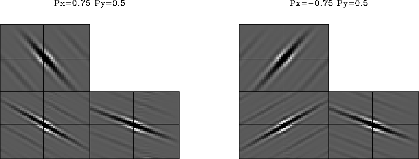
Figure 25 3-D plane wave construction with the factorized
3-D filter. Left:  ,
,  . Right:
 ,
,  .
.
![[*]](http://sepwww.stanford.edu/latex2html/movie.gif)


Figure ![[*]](http://sepwww.stanford.edu/latex2html/cross_ref_motif.gif) shows examples of plane-wave construction. The
two plots in the figure are outputs of a spike, divided recursively
(on a helix) by
shows examples of plane-wave construction. The
two plots in the figure are outputs of a spike, divided recursively
(on a helix) by  , where
  is a 3-D
minimum-phase filter, obtained by the Wilson-Burg factorization.
Clapp (2000a) has proposed constructing 3-D plane-wave
destruction (steering) filters by splitting. In Clapp's method, the
two orthogonal 2-D filters  and
and  are simply
convolved with each other instead of forming the
autocorrelation (
are simply
convolved with each other instead of forming the
autocorrelation (![[*]](http://sepwww.stanford.edu/latex2html/cross_ref_motif.gif) ). While being a much more efficient
approach, splitting suffers from induced anisotropy in the inverse
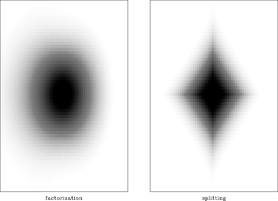
impulse response. Figure
). While being a much more efficient
approach, splitting suffers from induced anisotropy in the inverse
impulse response. Figure ![[*]](http://sepwww.stanford.edu/latex2html/cross_ref_motif.gif) illustrates this effect in the
2-D plane by comparing the inverse impulse responses of plane-wave
filters obtained by spectral factorization and splitting. The
splitting response is evidently much less isotropic.
illustrates this effect in the
2-D plane by comparing the inverse impulse responses of plane-wave
filters obtained by spectral factorization and splitting. The
splitting response is evidently much less isotropic.
bob
Figure 26 Two-dimensional inverse impulse
responses for filters constructed with spectral factorization (left)
and splitting (right). The splitting response is evidently much less
isotropic.


Next: 3-D missing data interpolation
Up: Plane-wave destruction in 3-D
Previous: Plane-wave destruction in 3-D
Stanford Exploration Project
12/28/2000
![[*]](http://sepwww.stanford.edu/latex2html/cross_ref_motif.gif) ) satisfies the following
system of partial differential equations:
) satisfies the following
system of partial differential equations:

![[*]](http://sepwww.stanford.edu/latex2html/cross_ref_motif.gif) ) describes plane waves on the
) describes plane waves on the
![]() slices and is completely equivalent to
equation (
slices and is completely equivalent to
equation (![[*]](http://sepwww.stanford.edu/latex2html/cross_ref_motif.gif) ). In its discrete form, it is represented as
a convolution with the two-dimensional finite-difference filter
). In its discrete form, it is represented as
a convolution with the two-dimensional finite-difference filter
![]() from equation (
from equation (![[*]](http://sepwww.stanford.edu/latex2html/cross_ref_motif.gif) ). Similarly, the second
equation transforms into a convolution with filter
). Similarly, the second
equation transforms into a convolution with filter ![]() , which
acts on the
, which
acts on the ![]() slices. The discrete (finite-difference) form of
equations (
slices. The discrete (finite-difference) form of
equations (![[*]](http://sepwww.stanford.edu/latex2html/cross_ref_motif.gif) ) involves a blocked convolution operator:
) involves a blocked convolution operator:
![[*]](http://sepwww.stanford.edu/latex2html/cross_ref_motif.gif) , regularization implicitly
deals with the spectrum of the regularization filter, which
approximates the inverse model covariance. In other words, it involves
the square operator
, regularization implicitly
deals with the spectrum of the regularization filter, which
approximates the inverse model covariance. In other words, it involves
the square operator
![]() from its spectrum is the familiar
spectral factorization problem. In fact, we already encountered a
problem analogous to (
from its spectrum is the familiar
spectral factorization problem. In fact, we already encountered a
problem analogous to (![[*]](http://sepwww.stanford.edu/latex2html/cross_ref_motif.gif) ) in the previous section in the
factorization of the discrete two-dimensional Laplacian operator:
) in the previous section in the
factorization of the discrete two-dimensional Laplacian operator:
![]() with the help of a simple first-order
upwind finite-difference scheme
with the help of a simple first-order
upwind finite-difference scheme

![[*]](http://sepwww.stanford.edu/latex2html/cross_ref_motif.gif) ) produces a minimum-phase
filter applicable for 3-D forward and inverse convolution.
Equation (
) produces a minimum-phase
filter applicable for 3-D forward and inverse convolution.
Equation (![[*]](http://sepwww.stanford.edu/latex2html/cross_ref_motif.gif) ) is shown here just to illustrate the concept.
In practice, I use the longer and much more accurate plane-wave
filters of equation (
) is shown here just to illustrate the concept.
In practice, I use the longer and much more accurate plane-wave
filters of equation (![[*]](http://sepwww.stanford.edu/latex2html/cross_ref_motif.gif) ) in place of the simplified
filters (
) in place of the simplified
filters (![[*]](http://sepwww.stanford.edu/latex2html/cross_ref_motif.gif) ) and (
) and (![[*]](http://sepwww.stanford.edu/latex2html/cross_ref_motif.gif) ).
).

![[*]](http://sepwww.stanford.edu/latex2html/movie.gif)
![[*]](http://sepwww.stanford.edu/latex2html/cross_ref_motif.gif) shows examples of plane-wave construction. The
two plots in the figure are outputs of a spike, divided recursively
(on a helix) by
shows examples of plane-wave construction. The
two plots in the figure are outputs of a spike, divided recursively
(on a helix) by ![]() , where
, where ![]() is a 3-D
minimum-phase filter, obtained by the Wilson-Burg factorization.
is a 3-D
minimum-phase filter, obtained by the Wilson-Burg factorization.
![]() and
and ![]() are simply
convolved with each other instead of forming the
autocorrelation (
are simply
convolved with each other instead of forming the
autocorrelation (![[*]](http://sepwww.stanford.edu/latex2html/cross_ref_motif.gif) ). While being a much more efficient
approach, splitting suffers from induced anisotropy in the inverse
impulse response. Figure
). While being a much more efficient
approach, splitting suffers from induced anisotropy in the inverse
impulse response. Figure ![[*]](http://sepwww.stanford.edu/latex2html/cross_ref_motif.gif) illustrates this effect in the
2-D plane by comparing the inverse impulse responses of plane-wave
filters obtained by spectral factorization and splitting. The
splitting response is evidently much less isotropic.
illustrates this effect in the
2-D plane by comparing the inverse impulse responses of plane-wave
filters obtained by spectral factorization and splitting. The
splitting response is evidently much less isotropic.
