Continuous Fourier basis

For the continuous Fourier transform, the set of basis functions is defined by  

$$\psi_\omega (x) = \frac{1}{\sqrt{2 \pi}} e^{i \omega x} \;,$$ (45)

where $\omega$ is the continuous frequency. For a 1-point sampling interval, the frequency is limited by the Nyquist condition: $\vert\omega\vert \leq \pi$. In this case, the interpolation function W can be computed from equation () to be  

$$W (x, n) = \frac{1}{2 \pi} \int_{-\pi}^{\pi} e^{i \omega (x... ...\omega = \frac{\sin \left[\pi (x - n) \right]}{\pi (x - n)} \;.$$ (46)

The shape of the interpolation function () and its spectrum are shown in Figure . The spectrum is identically equal to 1 in the Nyquist frequency band.

 

sincint
Figure 7 Sinc interpolant (left) and its spectrum (right).

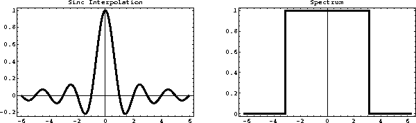Function () is well-known as the Shannon sinc interpolant. According to the sampling theorem Kotel'nikov (1933); Shannon (1949), it provides an optimal interpolation for band-limited signals. A known problem prohibiting its practical implementation is the slow decay with (x - n), which results in a far too expensive computation. This problem is solved in practice with heuristic tapering Hale (1980), such as triangle tapering Harlan (1982), or more sophisticated taper windows Wolberg (1990). One popular choice is the Kaiser window Kaiser and Shafer (1980), which has the form  

$$W (x, n) = \left\{\begin{array} {lcr} \displaystyle \frac{... ...n - N < x < n + N \\ 0, & \mbox{otherwise} &\end{array}\right.$$ (47)

where I₀ is the zero-order modified Bessel function of the first kind. The Kaiser-windowed sinc interpolant () has the adjustable parameter a, which controls the behavior of its spectrum. I have found empirically the value of a=4 to provide a spectrum that deviates from 1 by no more than 1% in a relatively wide band.

While the function W from equation () automatically satisfies properties () and (), where both x and n range from $-\infty$ to $\infty$, its tapered version may require additional normalization.

Figure  compares the interpolation error of the 8-point Kaiser-tapered sinc interpolant with that of cubic convolution on the example from Figure . The accuracy improvement is clearly visible.

 

cubkai Figure 8 Interpolation error of the cubic-convolution interpolant (dashed line) compared to that of an 8-point windowed sinc interpolant (solid line).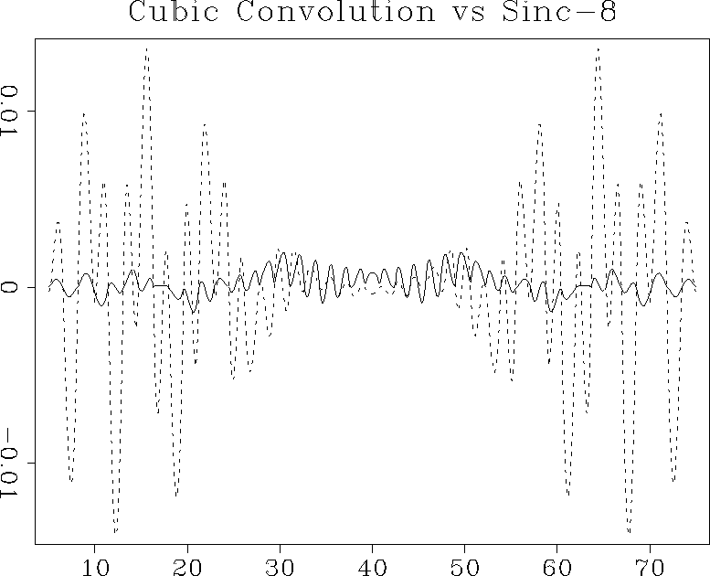

The differences among the described forward interpolation methods are also clearly visible from the discrete spectra of the corresponding interpolants. The left plots in Figures  and  show discrete interpolation responses: the function W(x,n) for a fixed value of x=0.7. The right plots compare the corresponding discrete spectra. Clearly, the spectrum gets flatter and wider as the accuracy of the method increases.

 

speclincub Figure 9 Discrete interpolation responses of linear and cubic convolution interpolants (left) and their discrete spectra (right) for x=0.7.

 

speccubkai Figure 10 Discrete interpolation responses of cubic convolution and 8-point windowed sinc interpolants (left) and their discrete spectra (right) for x=0.7.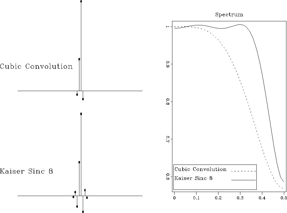