


Next: B-splines
Up: Forward Interpolation
Previous: Nearest neighbor and beyond
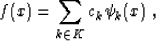
As I discussed in an earlier paper Fomel (1997b), a
general approach for constructing the interpolant function W(x,n) in
equation (1) is to select an appropriate function basis
for representing the function f(x). The functional basis
representation has the general form
|  |
(6) |
where  are basis function, and ck are the corresponding
coefficients. Once an appropriate basis is selected, one can define
the W(x,n) function by means of the least squares method.
are basis function, and ck are the corresponding
coefficients. Once an appropriate basis is selected, one can define
the W(x,n) function by means of the least squares method.
Unser et al. (1993a) noticed that the function basis idea has an
especially simple implementation if the basis is
convolutional and satisfies the equation
| 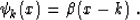 |
(7) |
In other words, the basis is constructed by integer shifts
of a single function  . Substituting
formula (7) into equation (6) yields
. Substituting
formula (7) into equation (6) yields
| 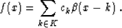 |
(8) |
Evaluating the function f(x) in equation (8) at an
integer value n, we obtain the equation
|  |
(9) |
which has the exact form of a discrete convolution. The basis function
, evaluated at integer values, is digitally convolved with
the vector of basis coefficients to produce the sampled values of the
function f(x). We can invert equation (9) to obtain the
coefficients ck from f(n) by inverse recursive filtering
(deconvolution). In the case of a non-causal filter  , an
appropriate spectral factorization will be
needed prior to applying the recursive filtering.
, an
appropriate spectral factorization will be
needed prior to applying the recursive filtering.
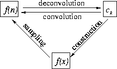
According to the convolutional basis idea, forward interpolation
becomes a two-step procedure. The first step is the direct inversion
of equation (9): the basis coefficients ck are found by
deconvolving the sampled function f(n) with the factorized filter
. The second step reconstructs the continuous (or arbitrarily
sampled) function f(x) according to formula (8). The
two steps could be combined into one, but usually it is more
convenient to apply them separately. I show a schematic relationship
among different variables in Figure ![[*]](http://sepwww.stanford.edu/latex2html/cross_ref_motif.gif) .
.
scheme
Figure 10 Schematic relationship among
different variables for interpolation with a convolutional basis.
|
|  |

Next: B-splines
Up: Forward Interpolation
Previous: Nearest neighbor and beyond
Stanford Exploration Project
9/5/2000