 |
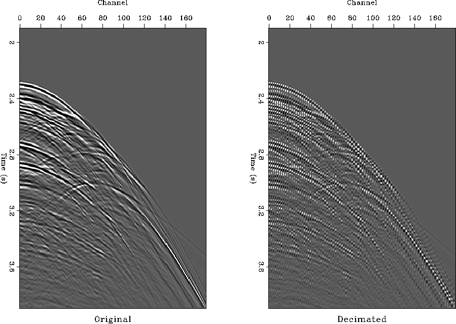
Figure 13 2-D marine shot gather. Left: original. Right: subsampled by a factor of two in the offset direction.
Spitz (1991) popularized the application of prediction-error filters to regular trace interpolation and showed how the spatial aliasing restriction can be overcome by scaling the frequencies of F-X PEFs. An analogous technique for T-X filters was developed by Claerbout (1992a, 1999) and applied for 3-D interpolation with non-stationary PEFs by Crawley (2000). The T-X technique implies stretching the filter in all directions so that its dip spectrum is preserved, while the coefficients can be estimated at alternating traces. After the filter is estimated, it is scaled back and used for interpolating missing traces in between the known ones. A very similar method works for finite-difference plane wave destructors, only we need to take a special care to avoid aliased dips at the dip estimation stage.
Figure 13 shows a marine 2-D shot gather from a deep water Gulf of Mexico survey before and after subsampling in the offset direction. The data are similar to those used by Crawley (2000). The shot gather has long-period multiples and complicated diffraction events caused by a salt body. Subsampling by a factor of two (the right plot in Figure 13) causes a clearly visible aliasing in the steeply dipping events. The goal of my first experiment was to interpolate the missing traces in the subsampled data and to compare the result with the original gather shown in the left plot of Figure 13.
 |
A straightforward application of the dip estimation equations (16-18) applied to aliased data can easily lead to erroneous aliased dip estimation. In order to avoid this problem, I chose a slightly more complex strategy. The algorithm for trace interpolation of aliased data consists of the following steps:
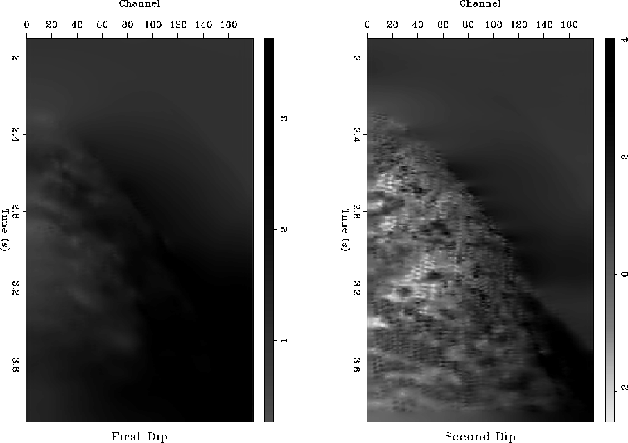 |
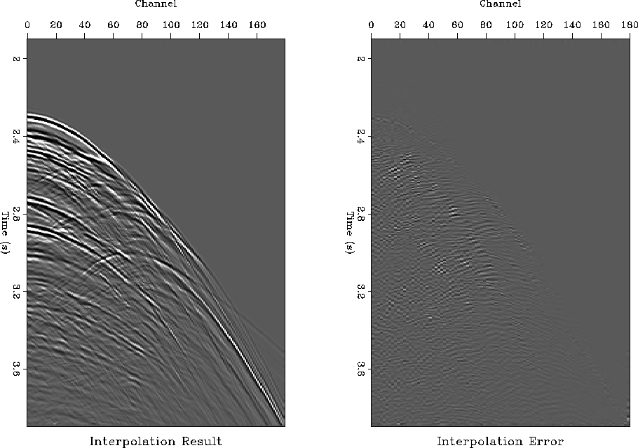
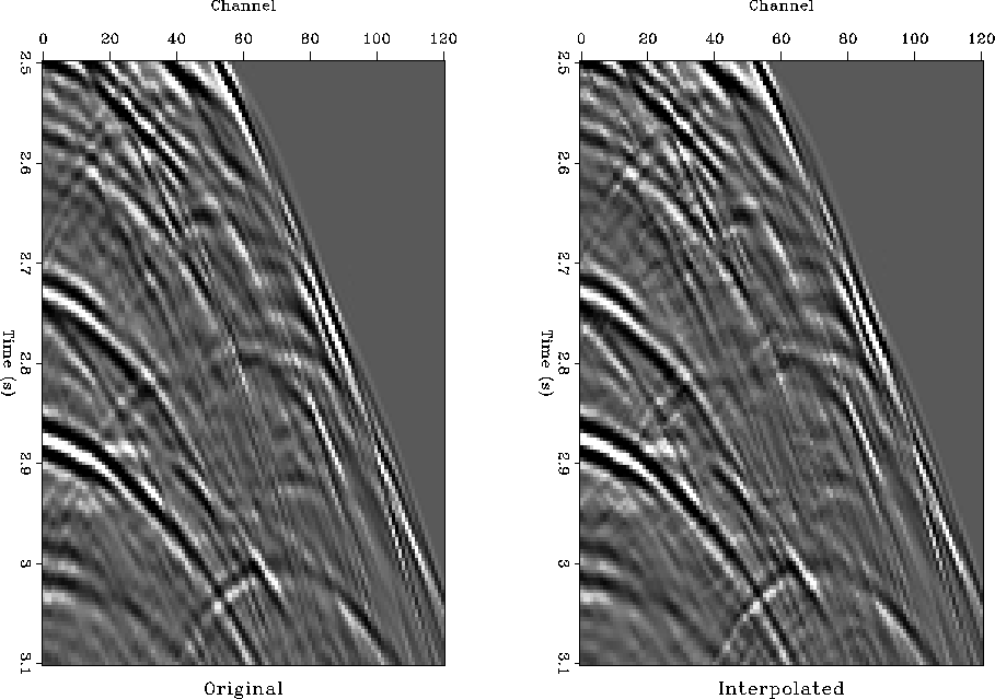
Figure 15 shows the interpolation result and the difference between the interpolated traces and the original traces, plotted at the same clip value. The method succeeded in the sense that it is impossible to distinguish interpolated traces from the interpolation result alone. However, it is not perfect in the sense that some of the original energy is missing in the output. A closeup comparison between the original and the interpolated traces in Figure 16 shows that imperfection in more detail. Some of the steepest events in the middle of the section are poorly interpolated, and in some of the other places, the second dip component is continued instead of the first one.
 |
 |
![[*]](http://sepwww.stanford.edu/latex2html/movie.gif)
The interpolation result can be considerably improved by including another dimension. To achieve a better result, we can use a pair of plane-wave destructors, one predicting local plane waves in the offset direction, and the other predicting local plane waves in the shot direction.