Next: Gap interpolation
Up: Application examples
Previous: Application examples
The use of prediction-error filters in the problem of detecting local
discontinuities was suggested by
Claerbout (1992b, 1993, 1999) and further
refined by Schwab et al. (1996a,b) and
Schwab (1998). Bednar (1997) used
simple plane-destructor filters in a similar setting to compute coherency
attributes.
To test the performance of the improved plane-wave destructors, I
chose several examples from Claerbout (1992b).
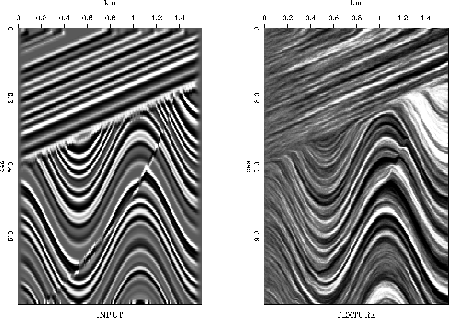
Figure 2 introduces the first example. The left
plot of the figure shows a synthetic model, which resembles
sedimentary layers with a plane unconformity and a curvilinear fault.
The right plot shows the corresponding ``texture''
Brown (1999); Claerbout and Brown (1999), obtained by
convolving a field of random numbers with the inverse plane-wave
destructor filters. The inverse filters were constructed with the
B-spline regularization technique Fomel (2000b), while
the dip field was estimated by the linearization method of the
previous section. The dip field itself and the prediction residual
[the left-hand side of equation (13)] are shown in the left
and right plots of Figure 3 respectively. We
observe that the texture plot does reflect the dip structure of the
input data, which indicates that the dip field was estimated
correctly. The fault and unconformity are clearly visible both in the
dip estimate and in the residual plots. Anywhere outside the slope
discontinuities and the boundaries, the residual is close to zero.
Therefore, it can be used directly as a fault detection measure.
Comparing the residual plot in Figure 3 with
the analogous plot of Claerbout (1992b) establishes a
superior performance of the improved finite-difference destructors in
comparison with that of the local T-X prediction-error filters.
txtr-sigmoid0
Figure 2 Synthetic sedimentary model. Left
plot: Input data. Right plot: Its texture.


 lomo2-sigmoid0
Figure 3 Synthetic sedimentary model. Left
plot: Estimated dip field. Right plot: Prediction residual.
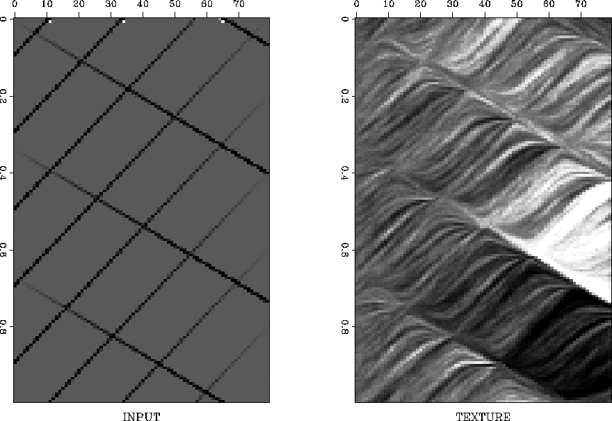
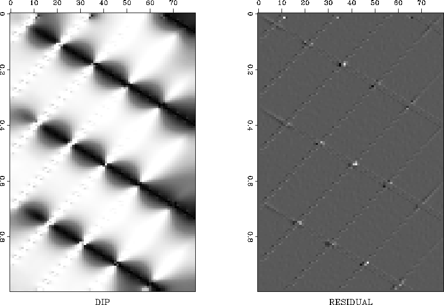
Figure 4 shows a simpler synthetic test. The
model is composed of linear events with two conflicting slopes. A
regularized dip field estimation attempts to smooth the estimated dip
in the places where it is not constrained by the data (the left plot
of Figure 5.) The corresponding residual (the
right plot of Figure 5) shows suppressed linear
events and highlights the places of their intersection.
txtr-conflict
Figure 4 Conflicting dips synthetic. Left
plot: Input data. Right plot: Its texture.
lomo-conflict
Figure 5 Conflicting dips synthetic. Left
plot: Estimated dip field. Right plot: Prediction residual.
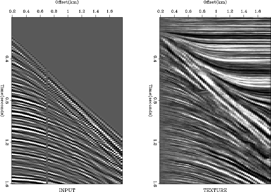
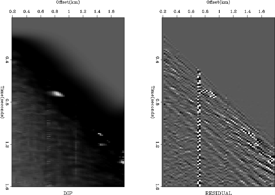
The left plot in Figure 6 shows a real shot gather
(a portion of Yilmaz and Cumro data set 27). The initial dip in the
dip estimation program was set to zero. Therefore, the texture image
(the right plot in Figure 6) contains zero-dipping
plane waves in the places of no data. Everywhere else the dip is
accurately estimated from the data. The data contain a missing trace at about 0.7 km
offset and a slightly shifted (possibly mispositioned) trace at about
1.1 km offset. The mispositioned trace is clearly visible in the dip
estimate (the left plot in Figure 7), and the
missing trace is emphasized in the residual image (the right plot in
Figure 7). Additionally, the residual image reveals
the forward and back-scattered surface waves, hidden under more
energetic reflections in the input data.
txtr-yc27
Figure 6 Real shot gather. Left
plot: Input data. Right plot: Its texture.
lomo2-yc27
Figure 7 Real shot gather. Left
plot: Estimated dip field. Right plot: Prediction residual.
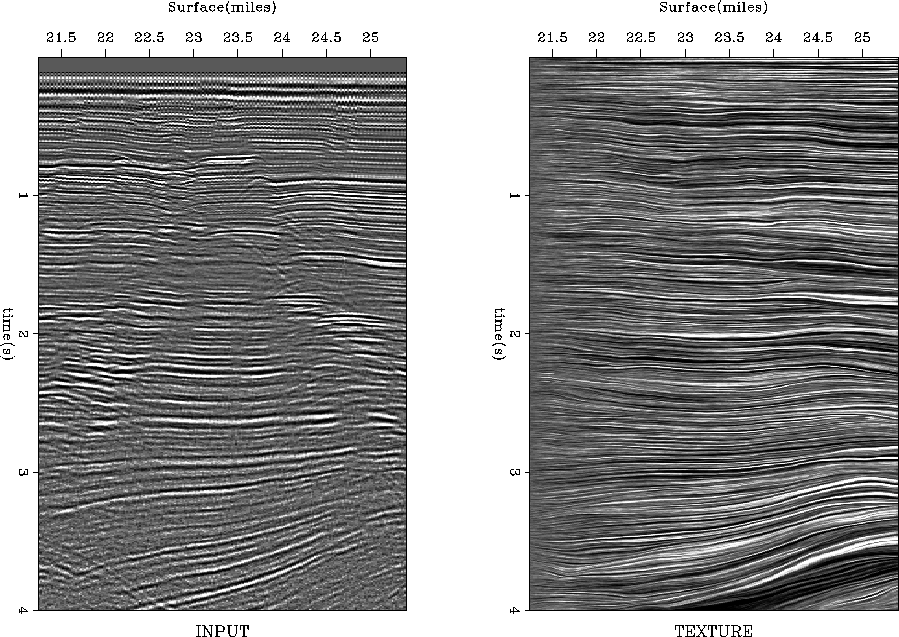
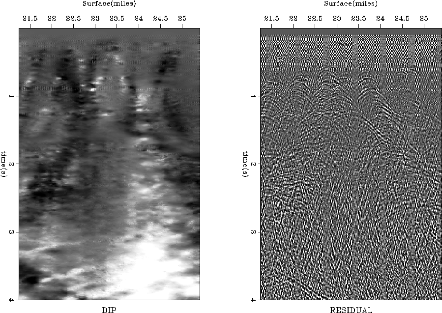
Figure 8 shows a stacked time section from the Gulf of
Mexico and its corresponding texture. The texture plot demonstrates
that the estimated dip (the left plot of Figure 9)
reflects the dominant local dip in the data. After the plane waves
with that dip are removed, many hidden diffractions appear in the
residual image (the right plot in Figure 9.) The
enhanced diffraction events can be used, for example, for
estimating the medium velocity Harlan et al. (1984).
txtr-dgulf
Figure 8 Time section from the Gulf of Mexico. Left
plot: Input data. Right plot: Its texture.
lomo-dgulf
Figure 9 Time section from the Gulf of Mexico. Left
plot: Estimated dip field. Right plot: Prediction residual.
Overall, the examples of this subsection show that the
finite-difference plane-wave destructors are a reliable tool for
enhancement of discontinuities and conflicting slopes in seismic
images. The estimation step of the fault detection procedure produces
an image of the local dip field, which may have its own
interpretational value. An extension to 3-D is possible, as outlined
by
Claerbout (1993), Schwab (1998),
Fomel (1999), and Clapp (2000a).
Next: Gap interpolation
Up: Application examples
Previous: Application examples
Stanford Exploration Project
9/5/2000