Imaging the location of seismic sources

The top panel of Figure 4 shows synthetic data generated for a point exploder embedded in a constant velocity medium centered 1050 m below a 2100 m wide array. There are 70 geophones in the array with a geophone spacing of 30 m. The traces are computed for 1 second of duration with a 30 Hz Ricker wavelet source. The point scatterer response of the Kirchhoff operator and the crosscorrelation migration operator in equation (4) are shown in the middle and lower panels of Figure 4, respectively.

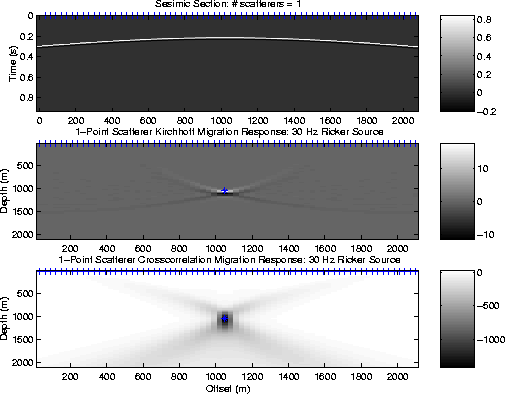
Note, the crosscorrelation image of the point scatterer is smeared over a larger depth range than that of the Kirchhoff image. This is because the crosscorrelation of one trace with another smears the source wavelet into a longer wavelet, and also because the crosscorrelation operator has poor resolution in the depth direction (see Figure 5). Nevertheless, the crosscorrelation point-scatterer image is acceptable.

In practice, the master trace and its two nearest neighbors were muted because the direct wave migration operator in equation (4) has zero or nearly zero phase when $g \approx g'$. This is undesirable because any energy from these traces will be smeared uniformly throughout the model, not just at the exploder points. Also, a second derivative in time was applied to the crosscorrelogram traces to partly compensate for the smoothing effects of crosscorrelation and migration.

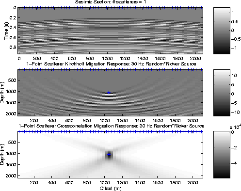
Figure 5 is the same as Figure 4 except the source wavelet is a long random time series. The crosscorrelation of traces collapses the ringy time series to an impulse-like wavelet so that the associated migration image in the lower panel of Figure 5 has good spatial resolution compared to the Kirchhoff image in the middle panel.

 

fig4
Figure 4 Source imaging test with 30 Hz impulsive source at a depth of 1050 m and t=0: The top panel shows the synthetic data. The middle panel shows the Kirchhoff migration image, and lower panel shows crosscorrelation migration image. The true image location is marked by an asterisk (*). The Kirchhoff image is better resolved than the crosscorrelation image partly because the temporal crosscorrelation broadens the seismic wavelet.

 

fig5
Figure 5 Same as Figure 4, except the source wavelet is a long random time series beginning at t=0. The top panel shows the synthetic data. The middle panel shows the Kirchhoff migration image, and lower panel shows crosscorrelation migration image. The true image location is marked by an asterisk (*). Note that the crosscorrelation of traces collapses the ringy source wavelet into an impulsive-like wavelet, leading to a better resolved migration image in the crosscorrelogram image.

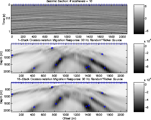
In the previous examples, the scatterer exploded at time zero. Figure 6 shows a similar synthetic experiment with ten scatterers, all exploding at random times with a random time series as a source wavelet. The resulting data for 1 second is shown in the top panel of Figure 6. The middle panel shows these data after crosscorrelation migration of 1 second of data, and roughly locates the location of the 10 point sources. Repeating this crosscorelation migration for fifteen data sets, each with 1 second of data generated from ten point scatterers with distinct random time histories, yields the stacked images shown in the lower panel of Figure 6. As expected, averaging the migration images tends to cancel migration noise and reinforce the energy at the location of the point exploders.

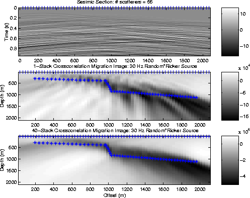
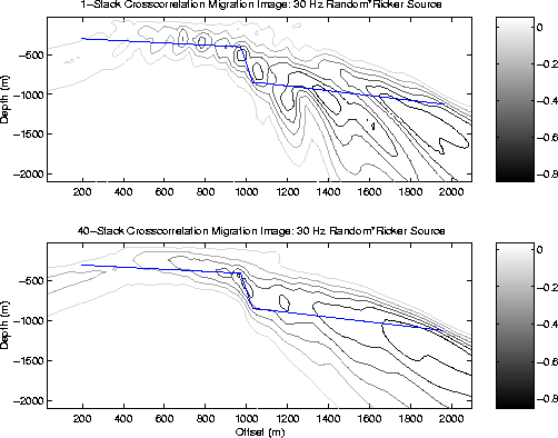
Finally, the fault-like structure denoted by stars in Figure 7 is assumed to emanate seismic energy randomly in time with random strength. This might approximate the situation where fluid is injected along a reservoir bed and seismic instruments are passively monitoring the injection front. Figure 7 shows the results after crosscorrelation migration of 1 second of data (middle panel), and 40 stacks of 1 second records (lower panel). The fault boundaries are much better delineated in the 40-stack migration image, although the resolution is much worse than that of an ordinary seismic survey.

Poor resolution of the crosscorrelation images is consistent with theoretical predictions of resolution for crosscorrelation migration operators. A possibility for improving resolution is to measure the incidence angle of energy in the correlograms and use this angle as a constraint in smearing data into the model. This strategy is similar to that of ray-map migration, but it remains to be seen if this is a practical strategy with correlograms.

 

fig6a
Figure 6 Similar to previous figures, except there are ten isolated random point sources (*). The top panel shows the synthetic data. The middle panel shows the crosscorrelation migrated image, computed from 1 second of data; while the bottom image shows the result after 15 stacks of 1-second data. The stacked image is better resolved because stacking tends to cancel noise and reinforce migration energy at the point exploder locations.

 

f7
Figure 7 (Top). Source imaging test with 55 point exploders located along a fault-like boundary. The points exploded at random times with random weighting amplitudes. The top panel shows the synthetic data. The middle panel shows the crosscorrelation migrated image, computed from 1 second of data; while the bottom image shows the result after 40 stacks of 1-second data. The stacked image appears to be less noisy and a better approximation to the fault geometry delineated by stars.

 

fb
Figure 8 Similar to previous figure except the migration images are contoured, and the fault boundary is delineated by a dashed line. The top panel shows the crosscorrelation migrated image, computed from 1 second of data; while the bottom image shows the result after 40 stacks of 1-second data.