The downward continued wavefield in Equation (6) can be rewritten as
| |
(13) |
| |
(14) |
| |
(15) |
When computed using the operator in Equation (15), the scattered wavefield,
Equation (14), exhibits a nonlinear relation to the
slowness perturbation. A straightforward linearization is to approximate
![]() for the constant background slowness.
Biondi and Sava (1999) implement the prestack version of
the scattering operator using a 4th order Taylor series expansion, under
the constant velocity assumption (
for the constant background slowness.
Biondi and Sava (1999) implement the prestack version of
the scattering operator using a 4th order Taylor series expansion, under
the constant velocity assumption (![]() and s=so) for all the terms
in the sum:
and s=so) for all the terms
in the sum:
| |
(16) |
|
sc
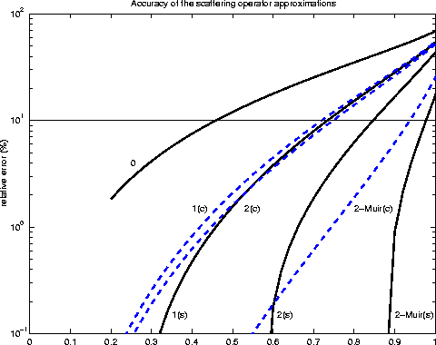
Figure 3 Comparison of various approximation for the linear scattering operator. The solid lines correspond to scattering operators computed using the spatially variable slowness function (s), and the dashed lines correspond to the scattering operator computed using only the background slowness (so). The accuracy of the operator improves when using the variable slowness function. The horizontal axis is the ratio |  |
Figure ![[*]](http://sepwww.stanford.edu/latex2html/cross_ref_motif.gif) shows a comparison of various approximation for the linear scattering
operator, Equation (15). As expected, the relative error of the backprojection operator
increases with increasing ratio
shows a comparison of various approximation for the linear scattering
operator, Equation (15). As expected, the relative error of the backprojection operator
increases with increasing ratio ![]() . Also, Muir's continuous fraction expansion gives a
significantly better approximation to the scattering operator for the same order of the
expansion. The solid horizontal line corresponds to
. Also, Muir's continuous fraction expansion gives a
significantly better approximation to the scattering operator for the same order of the
expansion. The solid horizontal line corresponds to ![]() relative error of the
approximate to the true scattering operator.
relative error of the
approximate to the true scattering operator.
After we apply the imaging condition to the downward continued scattered wavefield
Equation (13), we can formulate the relationship between the image (![]() ) and
slowness (
) and
slowness (![]() ) perturbations as
) perturbations as
| |
(17) |
Next section presents a simple example, in which I simulate ![]() and compute
and compute ![]() using a prestack backprojection operator derived from Equation (16).
using a prestack backprojection operator derived from Equation (16).