Well Interpolation

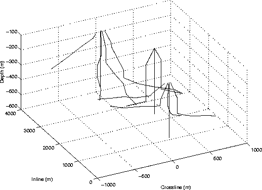
The data for this project was supplied by the rock physics group at Stanford University. It is from the Stanford V synthetic data set, which is a 3-D model set in a fluvial environment. The trajectories for the wells used in this project are displayed in Figure 2. The geometry represents wells from three separate platforms. In order to extract inline slices easier, the data was rotated $37^\circ$ to an inline azimuth of $0^\circ$ or directly north south, as shown in Figure 1.

 

rotated_wells
Figure 1 Rotated wells to N-S axis.

 

wells
Figure 2 Original orientation of well data.

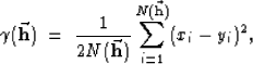
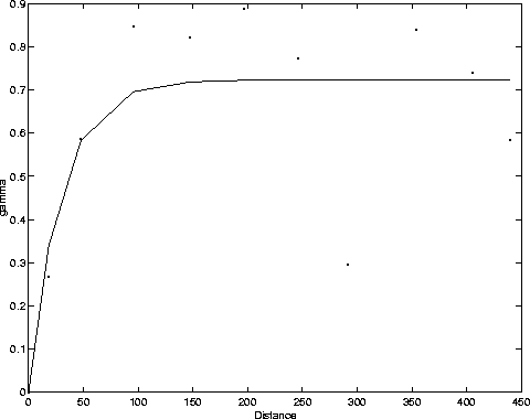
The interpolation between the wells was done using an ordinary kriging method. The actual operator is a part of the kt3d program in the GSLIB software package Deutsch and Journel (1998). The distance dependence of the kriging operator is found by looking at variograms. Variograms were calculated using the program gamv, another part of the GSLIB library. The horizontal variogram, Figure 3, shows better correlation at greater distances than the vertical variogram, Figure 4. This is expected because in a real geologic setting, rocks usually are deposited in roughly horizontal packages which usually are much wider than they are deep. The actual variogram was a semivariogram, which is commonly used to correlate two attribute values separated by a distance vector,

$$\gamma({\bf \vec{h}}) \; = \; \frac{1}{2N({\bf \vec{h}})}\sum_{i=1}^{N({\bf \vec{h}})} (x_i-y_i)^2, \;$$ (1)

where $N({\bf \vec{h}})$ is the number of attribute pairs, x_i is the start or head value, and y_i is the end or tail Deutsch and Journel (1998). Thus, typically the value $\gamma$ will be zero where a data point is, and increase sharply then flatten off at great distances where there is no correlation between the head and tail points. The data fitting lines are exponential fits, which were fit in the equation:

$$\gamma({\bf \vec{h}}) \; = \; c \cdot \left[ 1 - e^{-\frac{3h}{a}}\right], \;$$ (2)

where a and c are found using a non-linear least squares algorithm. These values are used in the kt3d program. The ordinary kriging program uses the kriging estimator in the following equation Journel (2000),

 

$$Z_{OK}(\vec{u}) \; = \; \sum_{\alpha=1}^{n} {\lambda_\alpha}^{(OK)}(\vec{u})Z(\vec{u}_\alpha). \;$$ (3)

Basically, the ordinary kriging operator estimates at each location $\vec{u}$ a mean. The variance specified in the program is the same everywhere, and is defined in the program using a and c from equation (3). The ability to re-estimate the mean at each point is what differs ordinary kriging from simple kriging. This ability makes the ordinary kriging a robust technique because the random function model can be rescaled at each point. The robustness makes ordinary kriging appropriate for this problem, since the data is sampled so sparsely. This brief discussion of variograms and ordinary kriging is based on the discussion in the software users guide Deutsch and Journel (1998).

 

hoz_var
Figure 3 Horizontal variogram.

 

vert_var
Figure 4 Vertical variogram.

Figure 5 shows the 2D velocity slices used for the AVO modeling and velocity modeling. The slices correspond to the  m and 300 m crossline value in Figure 1, respectively. In these slices the data are the most dense, and thus the kriging algorithm is the most accurate. The slices from the output was 30 points on the depth axis, and 160 points on the distance axis. This was too coarse for the modeling, so a linear interpolation program was used to make the model 300 by 2000 points.

 

slice
Figure 5 Slices from 3-D data cube used in the modeling.

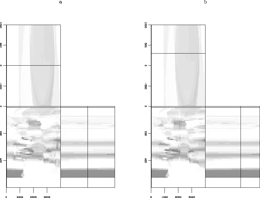The lateral velocity distribution around the well location in Figure 5b demostrate the stability of the interpolation operator because of the gradual lateral decay of the velocities and the absence of either vertical or horizontal fluctuations of the velocity distribution. It is not possible to asses the accuracy of the interpolation process because we do not have the original velocity model; however, the fact that it is possible to distinguish some bodies with lense shapes, which is a geological reasonable distribution of fluvial sedimentary environment, makes the model seen reasonable.