A cube of seismic data with an interesting set of dips was used as a test case. Half the traces were replaced by zeroes and input to four variations on the adaptive interpolation scheme of this chapter.
These tests use filters estimated in radial micropatches. The density of filters was chosen to give a good interpolation result, and to give patches that create an overdetermined problem at longer offsets and later times where the patches are largest, and an underdetermined problem where the patches are smaller.
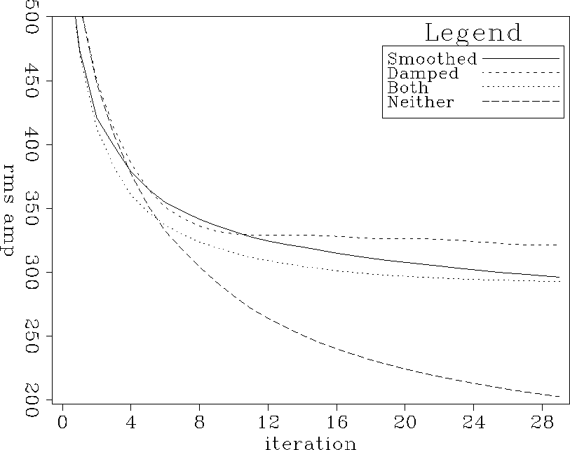
Figure curves.nrp shows the rms amplitude of the data-fitting residuals for the filter calculation step versus iteration number. The four curves correspond to four variations on the filter calculation scheme. The curve labels are:
The curves all start off about the same, with the three curves associated with any sort of smoothing and/or damping flattening out earlier and higher than the fourth. The residual of the filter calculation step goes down fastest when there is no restriction on the filters (the Neither curve). This is not surprising. Unfortunately, a small filter estimation residual is not necessarily good. In this case, it just means the filters have too many degrees of freedom.
The rms amplitude of the residual for the missing data calculation step is shown in Figure curves.nrd. A pleasing thing about all of these curves is that they converge after a handful of iterations. The empty spaces in the data are small, so they do not take long to fill in. Of course, some of the curves do not converge to very good answers; that depends on the PEFs calculated in the first stage.
|
curves.nrp
Figure 16 Filter calculation residual as a function of iteration. Curves represent different filter calculation schemes. |  |
|
curves.nrd
Figure 17 Missing data residual as a function of iteration. Curves represent different filter calculation schemes. |  |
Figure curves.nm shows the real quantity of interest. Each curve is the norm of the difference between the interpolated data and the true data as a function of iteration in the second step of the interpolation. The difference increases at some point in most cases. In principle the true data are unknown, and there is no reason for the difference not to increase. Significantly, the misfit starts to go up about the time that the residual from Figure curves.nrd bottoms out. The missing data residual bottoms out after about 6 iterations, and is guaranteed not to increase. The difference between the interpolated and true data begins to climb after the missing data problem has converged. Luckily, it does not climb very far.
The algorithm producing the curves labeled Smoothed
and that producing the curves labeled Both are closely related.
The former is just a special case of the latter, with ![]() With
With ![]() , there is no damping to control the null space
of the filter calculation step; control comes from not running
too many iterations.
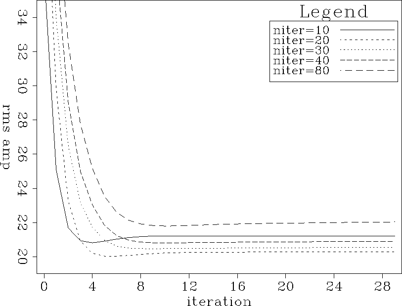
Figure curves.nm.filtniter shows how, with smoothing but
no damping, the number of iterations spent calculating filters
affects the misfit between the final interpolation result and the
true data.
The vertical axis is the sum of squares in the difference.
The horizontal axis is the number of iterations spent filling in
missing data.
The five curves correspond to different numbers of iterations
spent calculating filters.
For example, the curve labeled niter=30 shows the
rms amplitude of the difference between interpolated and true data as
a function of missing-data iteration, for the set of PEFs
calculated after 30 filter-calculation iterations.
As in Figure curves.nm, after a sufficient number of
missing data iterations,
the difference between interpolated and true data begins
to increase.
Figure curves.nm.filtniter shows that
the size of the misfit also goes up if too many iterations are spent
on the filter calculation.
After spending 80 iterations calculating PEFs,
the smallest possible result is
larger than if only 30 iterations were spent on the PEFs.
, there is no damping to control the null space
of the filter calculation step; control comes from not running
too many iterations.
Figure curves.nm.filtniter shows how, with smoothing but
no damping, the number of iterations spent calculating filters
affects the misfit between the final interpolation result and the
true data.
The vertical axis is the sum of squares in the difference.
The horizontal axis is the number of iterations spent filling in
missing data.
The five curves correspond to different numbers of iterations
spent calculating filters.
For example, the curve labeled niter=30 shows the
rms amplitude of the difference between interpolated and true data as
a function of missing-data iteration, for the set of PEFs
calculated after 30 filter-calculation iterations.
As in Figure curves.nm, after a sufficient number of
missing data iterations,
the difference between interpolated and true data begins
to increase.
Figure curves.nm.filtniter shows that
the size of the misfit also goes up if too many iterations are spent
on the filter calculation.
After spending 80 iterations calculating PEFs,
the smallest possible result is
larger than if only 30 iterations were spent on the PEFs.
Figures curves.nm.filtniter,
curves.nm.slightdamp.fn,
and
curves.nm.muchdamp
point to the utility of damping.
Figure curves.nm.slightdamp.fn shows the same
curves as are shown in Figure curves.nm.filtniter,
except that a small amount of damping is applied,
with ![]() .
That value was chosen by trial and error.
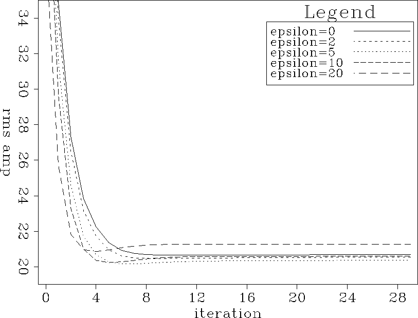
Figure curves.nm.muchdamp is also thematically similar
to Figure curves.nm.filtniter,
except that the number of filter calculation iterations
is held constant (at 30) and the value of
.
That value was chosen by trial and error.
Figure curves.nm.muchdamp is also thematically similar
to Figure curves.nm.filtniter,
except that the number of filter calculation iterations
is held constant (at 30) and the value of ![]() is incremented.
is incremented.
Figure curves.nm.slightdamp.fn shows that
choosing a reasonable value of ![]() helps to reduce the sensitivity of the final result to the
number of iterations in the filter calculation step.
Figure curves.nm.filtniter shows that increasing the number of iterations
from 30 to 80 with no damping causes a noticeable increase in the misfit,
While Figure curves.nm.slightdamp.fn shows that the same change in
number of iterations with damping has a smaller effect.
helps to reduce the sensitivity of the final result to the
number of iterations in the filter calculation step.
Figure curves.nm.filtniter shows that increasing the number of iterations
from 30 to 80 with no damping causes a noticeable increase in the misfit,
While Figure curves.nm.slightdamp.fn shows that the same change in
number of iterations with damping has a smaller effect.
Figure curves.nm.muchdamp shows that while
there is a choice between choosing the number of iterations
and choosing ![]() ,there appears to be an advantage to choosing
,there appears to be an advantage to choosing ![]() .Changing the number of iterations by a factor of about two
(again, from 30 to 80), with no damping,
showed a significant effect in Figure curves.nm.filtniter.
Changing the value of
.Changing the number of iterations by a factor of about two
(again, from 30 to 80), with no damping,
showed a significant effect in Figure curves.nm.filtniter.
Changing the value of ![]() by a larger factor
, while keeping iterations constant,
produces a very small effect in Figure curves.nm.muchdamp.
by a larger factor
, while keeping iterations constant,
produces a very small effect in Figure curves.nm.muchdamp.
|
curves.nm
Figure 18 Norm of the misfit between the true data and the interpolated data. Horizontal axis displays number of iterations in the missing data calculation step. Curves represent different filter calculation schemes. |  |
|
curves.nm.filtniter
Figure 19 Norm of the misfit between the true data and the interpolated data. Horizontal axis displays number of iterations in the missing data calculation step. Curves represent different numbers of iterations in the filter calculation step. |  |
|
curves.nm.slightdamp.fn
Figure 20 Norm of the misfit between true data and interpolated data. Curves represent different numbers of iterations in the filter calculation step. |  |
|
curves.nm.muchdamp
Figure 21 Norm of the misfit between true data and interpolated data. Curves represent different amounts of damping. |  |