


There are a couple of things to do about aliasing. In the 1-D case, the choices are bandpass filter the data before digitizing it, or live with it. With more dimensions come more possibilities, in particular the option to create more data. Most multichannel operators have some notion of operator antialiasing, which is essentially a bandpass on the impulse response of the operator, intelligently applied so that the maximum frequency is only as low as it has to be, changing with the dip of the operator.
Data aliasing can also, of course, be dealt with by bandpassing, but it would be foolish to throw away the useful information contained in the high frequencies. An alternative is to make more data. Aliasing in seismic data can almost always be thought of as not having traces spaced closely enough, along some axis. Interleaving a set of appropriately synthesized traces removes the problem without giving up the high frequencies. Naively interleaving traces (for instance by linear interpolation or by FFT and zero pad), will produce more data but with incorrect dips.
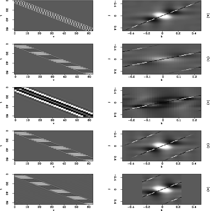
A simple example is shown in Figure introex. An almost-aliased diagonal event and its Fourier transform appear in Figure introexa. When the data are reduced to every second trace (introexb), the data are obviously aliased, such that the dipping event appears to be a series of horizontal events. The Fourier transform exhibits the expected wraparound. Bandpassing removes the aliasing wraparound, as shown in Figure introexc, but is not an attractive option because half the information is gone. Linear interpolation, shown in Figure introexd, extrapolates both the desired energy and the aliases in the frequency domain, so that the resampled data have the wrong dip. Zero padding in the frequency domain gives a similarly bad result. This is an excellent method when the data are not aliased. When the data are aliased, it does not really accomplish anything, as shown in Figure introexe. Restoring the data so that it looks like Figure introexa requires ``unwrapping'' the aliased energy visible in the second row, and not just zeroing or extrapolating it.
 |


A number of algorithms exist that attempt to do exactly that, with varying degrees of success, expense, and robustness. The most well known is the (f,x) interpolation method of Spitz . At each frequency, a spatial prediction filter is calculated from the known data, absorbing a set of constant linear dips to represent the data. A given filter is then used as an interpolation operator at double the frequency, where the spectrum it has captured from the known data corresponds to the same linear slopes at half the trace spacing.
A similar method is described by Claerbout Claerbout and Nichols (1991); Claerbout (1992b) , who estimates a PEF in the (t,x) domain and uses it as the interpolation operator. Where the frequencies are scaled in Spitz's (f,x) method, here Claerbout scales the physical axes of the PEF. The lag of a filter coefficient is scaled equally along all axes in order to represent the same slope at different trace spacings.
Basic to both of these methods is the assumption that seismic data are made up of linear events with constant slopes. This is clearly untrue for any large amount of data. Changes in structure, velocity, offset and time cause changes in the slope of seismic events. To get around this problem, we typically divide the data into small regions (from here on referred to as patches) where we assume that the data do have constant slopes. We estimate filters and interpolate traces in each patch. At the end we reassemble the patches, usually with some reasonable amount of overlapping, to make a full dataset.
Another group of methods are based on local Radon transforms. These methods make a similar assumption to the linear event assumption that the filtering methods above make, though whether the events are really assumed to be linear, parabolic, hyperbolic or whatever, depends on the particular Radon transform being used. In this case the Radon transform is the estimate of local dip, and the modeling adjoint of the transform stacking operator is the interpolator. Cabrera 1984 and Hugonnet 1997 describe variations on this theme. Novotny 1990 instead picks the strongest dip in the transform and linearly interpolates along it.
All the methods listed above are two-step methods, where the first step is to gather local information from regions of the data, and the second step is to use the information to synthesize new data with similar properties. Still another group of methods exist, which are based on migration-like operators. For example, Ronen 1987 applies DMO and inverse DMO iteratively to regrid spatially aliased data, and Chemingui 1996 uses AMO.