Parameter space

The parameters for smoothing and micropatching, the size and shape of the PEFs, and the number of iterations to spend on filter calculation and missing data calculation all make for a large parameter space. And unfortunately, results tend to be sensitive to at least a few of the parameters.

The numbers of iterations are important parameters, especially the number of filter calculation iterations. Too many iterations during the filter calculation step results in a noticeably degraded final result. A small amount of damping is very good at reducing sensitivity to the numbers of iterations, though the damping parameter $\epsilon$must be chosen, and a bad choice can also contribute to a bad result. Either way, a little experimentation usually will provide the answer. Most of the examples in this and the next chapter are done with $\epsilon=0$.

The size, shape, and density of PEFs can also lead to bad final results, if chosen poorly. In my experience the effectiveness of a set of filter parameters is largely independent of the lengths of the slow axes (shot number, midpoint number, etc.) of the input data. Put another way, the settings that work for one or two input gathers will generally work for any number of gathers, so it easy to test parameters quickly.

Another parameter that can significantly affect the outcome is the ratio of original spacing to interpolated spacing. In principle, it can be any integer, but in practice it should usually be two (as it is in most of the examples). There is no reason not to interpolate several times in a row, and this is usually the best way to get some larger ratio of sampling intervals. One reason is that scaling the axes of a PEF by a large factor decreases the range of frequencies that the PEF can reliably detect. The fix is to resample the time axis of the data, but that also means lengthening the PEF in time, in order to maintain the same range of dips. The extra degrees of freedom in the longer filter can result in spurious events and so forth. Even in simple tests, where the data is low frequency and does not require temporal resampling, my experience has been that interpolating in multiple steps works better than quadrupling (or more) the data in one step. As an example, Figure curtlow compares interpolation results where some very low frequency data have their offset sampling density quadrupled in two steps and in one step. The left panel shows the original data. The original data were lowpassed so that energy would lie below one quarter of its temporal Nyquist. The center panel shows the result of interpolating twice, doubling the data each time. The right panel shows the result of interpolating a single time, quadrupling the data. Something has obviously gone wrong in the right panel.

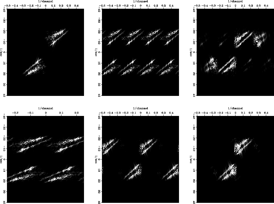
Figure curtlowspecs shows what happens in Fourier space. All the panels in this figure are cropped on the temporal frequency axis for clarity. The top left panel is the 2-D Fourier transform of the original, well-sampled data. The top center panel is the Fourier transform of the data after replacing three out of four traces with zeros. Zeroing the traces is a sampling operation, which leads to replication in the Fourier domain. The top right panel is the Fourier transform after attempting to interpolate all the zero traces at once. The interpolator needs to zero all the replicate versions of the input data's spectrum, and leave the originals alone. However, PEF spectra tend to be very simple (as in Figures diagonalin2 and diagonalout2), since a PEF is made up of a handful of coefficients. The PEF that passes the original part of the spectrum also passes the replicate spectrum that is aligned approximately along the same diagonal line in Fourier space. The two blobs in Fourier space that line up with the original data spectrum are only partially attenuated in the top right panel. Those events correspond to the same temporal frequencies, but higher wavenumbers, and so in the time domain the result has anomalously high dips (shown in the right panel in Figure curtlow).

The bottom three panels of Figure curtlowspecs, show the process of interpolating in two steps. The bottom left panel is the Fourier transform of the data with zero traces, after removing half the zeros. This panel is just like the top center, with the outermost spatial frequencies removed. In this case there is no trouble with original and replicate spectra aligning, and it is straightforward to interpolate. The bottom center panel shows the halfway point in the two steps of interpolation. This is the Fourier transform after interpolating and then reinserting the zeros that were removed. Again there is a replicate of the original spectrum to remove, but it does not line up with the original, so it is straightforward to remove it. The Fourier transform of the interpolation result is in the bottom right panel, the result in the time-domain is shown at the right side of Figure curtlow.

Manin and Spitz 1995 may allude to something similar, when they suggest that if fold is very low, the data should be interpolated in multiple steps along different directions.

 

curtlow
Figure 4 The difference between refining data sampling in one step and in multiple steps. The data in the left panel were subsampled by keeping every fourth offset, and zeroing the other three. The center panel shows the result of interpolating the data in two steps. The right panel shows the result of interpolating the data in one step.

 

curtlowspecs
Figure 5 Fourier transforms illustrating the difference between refining data in one step and in multiple steps. The top left is the spectrum of the original data. The top center is the spectrum after replacing three fourths of the traces with zeroes. The top right is the result of interpolating all the empty traces at once, it is not a good facsimile of the original spectrum at top left. The bottom left is the spectrum after removing two thirds of the zero traces. The bottom center is the spectrum after interpolating the remaining zero traces, and reinserting the zero traces which were removed. The bottom right is the spectrum of the final interpolation, and it is a much better estimate of the top left panel.