 |
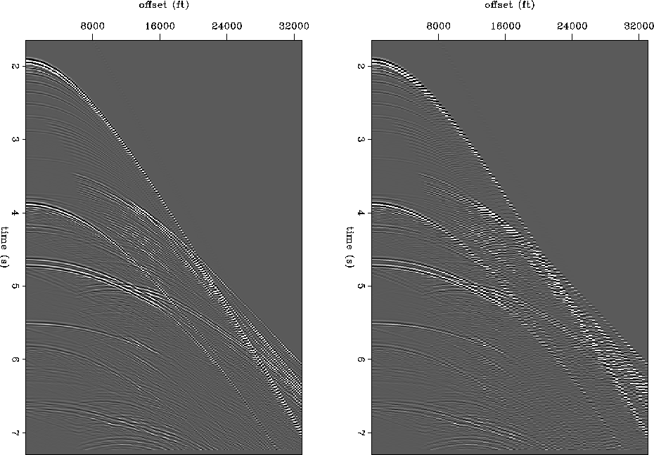
Figure 16 CMP gathers from the BP synthetic. The left panel is constructed from the full data set, the right is constructed from the subsampled data.
The data are modeled with equal source and receiver spacings. We can throw out every other shot, and thus simulate a single inline from a multi-source 3D survey. Alternatively, we can throw out every other receiver surface location, which in this case happens to be more convenient, but has the same effect on CMP sampling. As an example, Figures stackingchart1 and stackingchart2 show the difference in CMP sampling for a survey with equal shot and receiver sampling, and with the shot sampling interval doubled. Instead of removing rows from Figure stackingchart1 (as we did to make Figure stackingchart2), we could remove columns, and the CMP gathers would be undersampled in the same way. With half the data removed, the CMP gathers lose alternating offsets, so that the offset spacing is four times the offset spacing of a shot gather. The decrease in sampling causes many of the events to become aliased. Figure cmps1a shows a CMP gather constructed from the original data, with shot spacing equal to receiver spacing, and Figure cmps1b shows the CMP gather for the same midpoint, constructed from the subsampled input. This data contains apparently asymmetric events which make it appear not to be a CMP gather at all (for example at 5 seconds and 5000 meters offset), but these are peg-leg multiples with multiple paths, which would turn out to be symmetric if the negative offsets had been modeled. The mechanism is explained in detail by Thorson 1984. The steep events, which are not aliased or just slightly aliased in Figure cmps1a, are strongly aliased in Figure cmps1b. While the data do appear to be somewhat aliased in the Figure cmps1a, applying a slight moveout removes the aliasing. Moving out the data in the right panel does not remove the aliasing, because events curving upward begin to be aliased before events curving downwards cease to be aliased. Figures cmps1nmoa and cmps1nmob show the same two panels with moveout applied. The velocity chosen is between the primary and multiple velocity, so that on average everything will be relatively flat (not stackably flat, but hopefully flat enough that they are not aliased). The left panel, Figure cmps1nmoa, does not appear to be aliased at all, but in Figure cmps1nmob some of the events curving up and some of the events curving down have ambiguous dips.
 |
 |
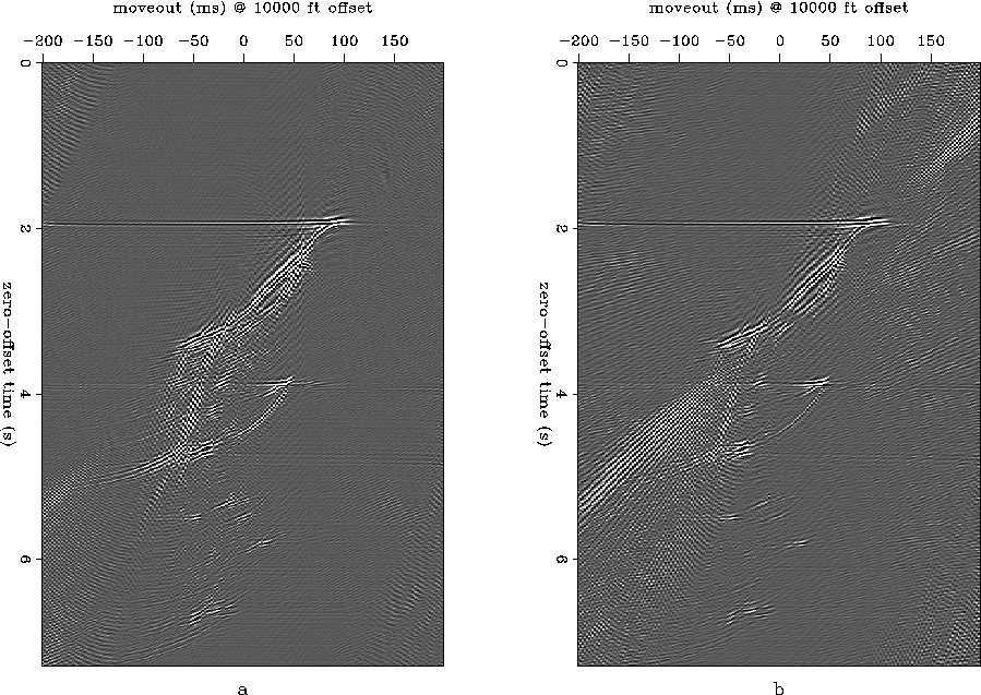
The dip ambiguity in Figure cmps1nmob leads to artifacts in the Radon transform. Parabolic Radon transforms of both panels appear in Figure rads1. Figure rads1a shows the Radon transform of the unaliased gather from cmps1nmoa, and Figure rads1b shows the Radon transform of the aliased gather from cmps1nmob. The horizontal axis displays milliseconds of moveout at 10000 feet of offset, rather than velocity or slowness. There are obvious artifacts, due to aliasing, streaking across Figure rads1b. These artifacts make it difficult to remove multiples, because energy from both primaries and multiples is spread throughout the Radon transform domain.
 |
The goal of the interpolation in this case is to generate dealiased data from the aliased data so that we wind up with a Radon transform similar to Figure rads1a and not Figure rads1b.