Marmousi synthetic

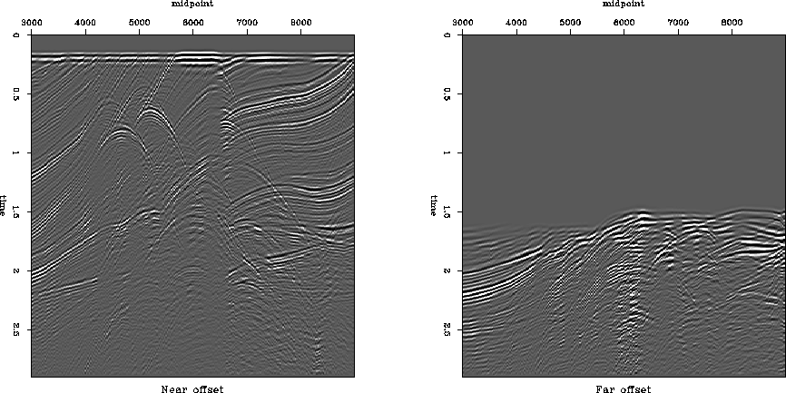
The famous Marmousi synthetic was modeled over a very complicated velocity and reflector structure Versteeg (1994). The dataset has been used in numerous studies of various seismic processing and imaging techniques. Figure 6 shows the near and far common-offset gathers from the Marmousi dataset. The structure of the reflection events is extremely complex and contains multiple triplications and diffractions.

 

marm
Figure 6 Common-offset gathers of the Marmousi dataset. Left: near offset. Right: far offset.

To test the proposed interpolation method, I set the goal of interpolating the missing near offsets in the Marmousi dataset. Additionally, I attempted to interpolate intermediate shot gathers so that all common-midpoint gathers receive the same offset fold. In the original dataset, both receiver and shot spacing are equal to 25 meters, which creates a checkerboard pattern in the offset-midpoint plane. This acquisition pattern is typical for 2-D seismic surveys.

Interpolation of near offsets can reduce imaging artifacts in different migration methods. Ji (1995) used near-offset interpolation for accurate wavefront-synthesis migration of the Marmousi dataset. He developed an interpolation technique based on the hyperbolic Radon transform inversion. Ji's method produces fairly good results, but is significantly more expensive that the offset continuation approach explored in this paper.

Figure 7 shows the input and interpolated Marmousi data in the log-stretch frequency domain. We can see that the data in the frequency slices also have a very complicated structure. Nevertheless, the offset continuation method is able to reconstruct the missing portions of the data in a visually pleasing way. The data are not extrapolated off the sides of the common-offset gathers. This behavior is physically reasonable, because such an extrapolation would involve assumptions about unilluminated portions of the subsurface.

 

mslice
Figure 7 Interpolation of the Marmousi dataset in frequency slices. Left: input data. Right: interpolation output. Top, center, and bottom plots correspond to different frequencies. Real parts of the complex-valued data are shown.

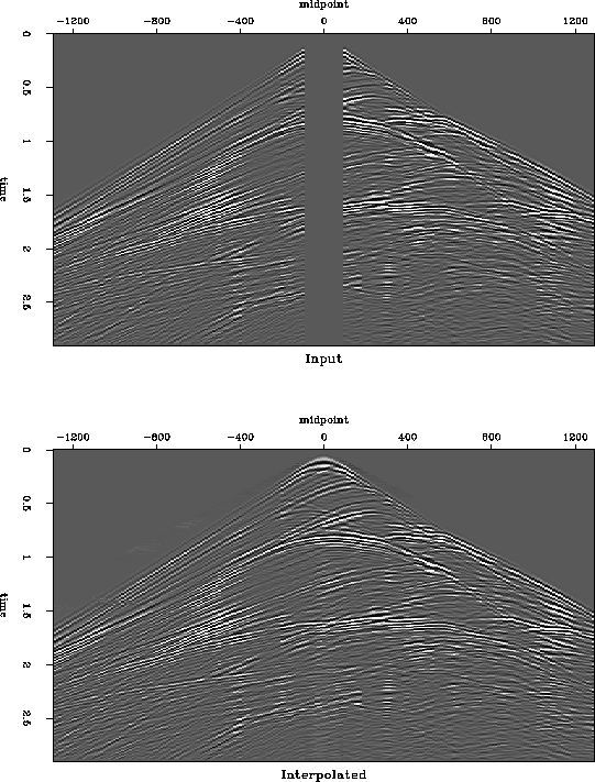
Figure 8 shows one of the shot gathers obtained after transforming the data back into time domain and resorting them into shot gathers. The positive offset part of the shot gather was reconstructed from a common receiver gather by using reciprocity. Comparing the top and bottom plots, we can see that many different events in the original shot gather are nicely extended into near offsets by the interpolation procedure.

 

mshot
Figure 8 Interpolation of near offsets in a Marmousi shot gather. The shot position is 4500 m. Top: input data. Bottom: interpolation output.

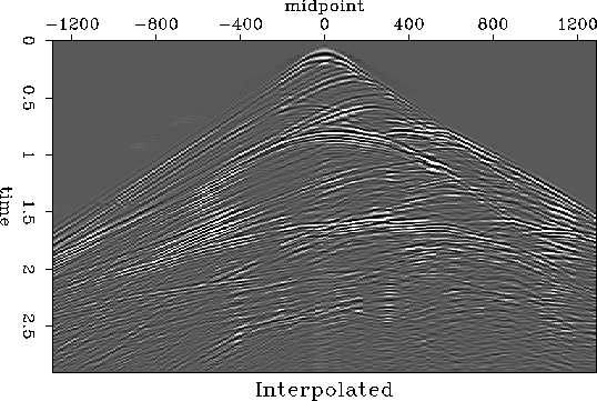
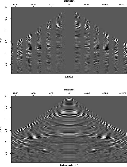
In addition to interpolating near offsets, I have reconstructed the intermediate shot gathers in order to equalize the CMP fold. Figure 9 shows an example of an artificial shot gather created by such a reconstruction. An sample CMP gather before and after interpolation is shown in Figure 10. Examining the bottom part of the section, we can see that that the interpolation process tends to put more continuity in the near offsets than could be expected from the data. In other places, the interpolation succeeds in producing a visually pleasant result.

 

mishot
Figure 9 This shot gather at 4525 m is a result of data interpolation.

 

mcmp
Figure 10 Interpolation of near and intermediate offsets in a Marmousi CMP gather. The midpoint position is 4500 m. Top: input data. Bottom: interpolation output.