Theory review

Stolt residual migration is formulated both for post-stack and prestack data. Stolt 1996 shows that, for the post-stack case, the residual migration operator is a function of the difference between the squared values of the original velocity and the new velocity to which the image is residually migrated. However, Stolt shows that such a formulation is no longer possible in the prestack case.

Sava (1999a,b) reformulates Stolt residual migration for depth-migrated images and shows that the operator is a function of the ratio of the two velocities, before and after residual migration, a formulation that holds for both post-stack and prestack (2-D, 3-D and common-azimuth) data.

In the 3-D case, the residual migration equation takes the form  

$$\begin{array} {r} k_z= \frac{1}{2}\sqrt{\frac{\v_0^2}{\v^2}... ...0^2}- \left\vert{\vec k_m}+{\vec k_h}\right\vert^2},\end{array}$$ (1)

where

• k_z0 and k_z are depth wavenumbers before and after residual migration,
• $\v_0$ and $\v$ are, respectively, the reference and the target migration velocities, and
• ${\vec k_m}$ and ${\vec k_h}$ are the offset and midpoint wavenumbers.

 

dipsynt.slo Figure 1 The slowness map used for the first 2-D synthetic examples.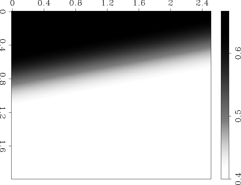

Strictly speaking, Equation (1) is derived from the constant velocity dispersion relations for pre-stack data. However, since the new images do not depend on the true magnitude of the new velocity, but rather on its ratio to the original, we can still techniquely apply residual migration, even when the original velocity is variable. The question is how valid such a residual migration operation is for the case of variable velocity, and whether the output provides any valuable information. A theoretical answer is not straightforward, since most likely the answer is data-dependent. I will, therefore, address the problem in an experimental way, first on synthetic models, and then on a North Sea real dataset.