


|
hector-dat
Figure 3 2-D shot gather. | 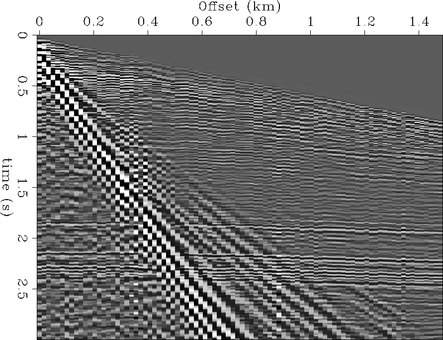 |


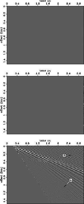
Figure 4 shows the RTT of the data in Figure 3 for both implementations. Each panel contains 300 radial traces. As mentioned by Henley (1999), the origin of the RTT can be placed anywhere. Often in land surveys, the near-zero offset traces are not recorded, meaning that the apparent origin of radial events will lie off the section. The following results were obtained with the the origin of the RTT placed at 0.25 seconds. As expected, the raw v-interpolation panel has many ``holes'', while the x-interpolation panel does not. The missing data estimation algorithm described above has plausibly filled the missing data, insofar as visual similarity to the x-interpolation panel is a valid measure.
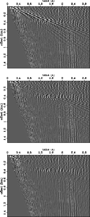
Figure 5 compares the error arising from both implementations of
the RTT (equation (3). In the RTT panels shown in Figure
4, each containing 300 radial traces, the error in both of the
v-interpolation panels is negligible. This figure gives visual proof of the fact that the
missing data infill process does not harm the original data, i.e., that the missing data points
in RT space are in the nullspace of ![]() . As expected, the x-interpolation error is nonzero,
particularly for high-wavenumber events like ground roll and likely backscatter.
Additionally, and less obviously, the primary events between 1.75 and 2.5 seconds suffer
energy loss and a noticeable lateral smoothing as a result of the transform.
. As expected, the x-interpolation error is nonzero,
particularly for high-wavenumber events like ground roll and likely backscatter.
Additionally, and less obviously, the primary events between 1.75 and 2.5 seconds suffer
energy loss and a noticeable lateral smoothing as a result of the transform.
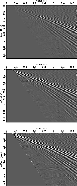
Figure 6 is the estimated signal (equation (8)). Notice that missing data infill has markedly improved the quality of noise suppression obtained by the v-interpolation technique. Still, by visual inspection, we must conclude that the x-interpolation result is the best of the three for noise suppression.
Figure 7 is the estimated noise (equation (9)). First notice that x-interpolation result contains more than just the radial ground roll that the simple physical model accounts for. From Figure 5, we know that the presence of the primary energy between 1.75 and 2.5 seconds and backscattered noise in the x-interpolation panel is due to interpolation errors, and not to the highpass filtering. The non-infilled v-interpolation result contains some energy (either artifacts or primary energy) around 1 second, while the infilled result does not. From the standpoint of signal preservation, the v-interpolation result with missing data infill is the best of the three. Philosophically, by using a pseudo-unitary RTT operator and thus ensuring that the only thing modifying the original data is the bandpass filter, the v-interpolation implementation honors the physics which drives the problem in the first place.
 |
![[*]](http://sepwww.stanford.edu/latex2html/movie.gif)
 |
 |
 |