|
schem
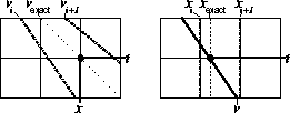
Figure 2 Left: ``v-interpolation'' implementation. Right: ``x-interpolation implementation. |  |
|
schem
Figure 2 Left: ``v-interpolation'' implementation. Right: ``x-interpolation implementation. |  |
In the v-interpolation approach, ![]() ``pushes'' energy -- weighted by linear interpolation
coefficients -- from fixed (t,x) bins into the two radial trace (t,v) bins that bracket them.
This implementation will cause interpolation error in regions where many (t,x) bins lie between
adjacent radial traces (see Fig. 1).
However, the RT domain is nonphysical in the sense that as many radial traces can be
used as computer memory permits, so the interpolation error can essentially be driven to zero
by sampling densely enough in RT space. Unfortunately, by sampling finely, in many
regions of RT space there are pairs of radial traces which bracket no (t,x) bin, so
``holes'' are introduced into the RT space which inhibit later filtering operations.
``pushes'' energy -- weighted by linear interpolation
coefficients -- from fixed (t,x) bins into the two radial trace (t,v) bins that bracket them.
This implementation will cause interpolation error in regions where many (t,x) bins lie between
adjacent radial traces (see Fig. 1).
However, the RT domain is nonphysical in the sense that as many radial traces can be
used as computer memory permits, so the interpolation error can essentially be driven to zero
by sampling densely enough in RT space. Unfortunately, by sampling finely, in many
regions of RT space there are pairs of radial traces which bracket no (t,x) bin, so
``holes'' are introduced into the RT space which inhibit later filtering operations.
In the x-interpolation approach, ![]() ``pulls'' energy into fixed (t,v) bins from the two
offset (t,x) bins that bracket them.
The interpolation error of this implementation depends only on the trace spacing of the data.
The net effect of applying the operator is to smooth laterally, making this implementation
dangerous if the data has even small static shifts.
At typical trace spacing,
``pulls'' energy into fixed (t,v) bins from the two
offset (t,x) bins that bracket them.
The interpolation error of this implementation depends only on the trace spacing of the data.
The net effect of applying the operator is to smooth laterally, making this implementation
dangerous if the data has even small static shifts.
At typical trace spacing, ![]() is not pseudo-unitary, but since the RT space is guaranteed to have
no ``holes'', this implementation is appropriate for post-filtering operations.
Henley (1999) used the x-interpolation approach, as did the author of the
SEPlib program Radial.
is not pseudo-unitary, but since the RT space is guaranteed to have
no ``holes'', this implementation is appropriate for post-filtering operations.
Henley (1999) used the x-interpolation approach, as did the author of the
SEPlib program Radial.
The two implementations of the RTT discussed above illustrate a fundamental, and oft-ignored duality in the analysis of interpolation operators. Intuition supports the x-interpolation method -- any given unknown model point is the weighted average of the two known data points which bracket it. In applications like NMO, where averaging is done along the well-sampled time axis, this intuition is sensible, but it breaks down when the averaging is across offsets. The alternate approach (v-interpolation) is less intuitive, as the interpolation is done across radial traces, in the ``virtual'' space of the model. Since the model space is not constrained by the parameters of data acquisition, it can be sampled as densely as needed to minimize interpolation error. In fact, in the limit of infinitely dense sampling in model space, simple nearest neighbor binning drives interpolation error to zero.
The idea of this paper is to use the v-interpolation RTT to take advantage of its minimal interpolation error, and then handle the problem of ``holes'' in RT space by missing data estimation. Ideally, the seismic gather contains nearly-horizontal primary reflections and radial events, so the RT space is composed of nearly-vertical (h(v)) and nearly-horizontal (l(t)) events which a cascade of derivative operators extinguishes:
| |
(4) |
| |
(5) |
| |
(6) | |
| (7) |
In this paper, we seek to use the RTT to do noise suppression. Specifically, we map a 2-D
seismic gather to RT space, then apply a conservative (6.5 Hz cutoff) highpass filter -
call it ![]() - to remove the noise, and finally transform back to (t,x) space. In
symbols, we can write the estimated signal,
- to remove the noise, and finally transform back to (t,x) space. In
symbols, we can write the estimated signal, ![]() , as follows
, as follows
| |
(8) |
| |
(9) |